• Posted on October 16, 2020
• Unique Submission Team

HA1011 Assignment 2020

 

1. Frequency distribution using 10 classes, stating the Frequency, Relative Frequency, Cumulative Relative Frequency and Class Midpoint.

 

Summary Statistics and Graphs
Mean	954.3667
Standard Error	90.65369
Median	715
Mode	401
Standard Deviation	702.2005
Sample Variance	493085.5
Kurtosis	1.604551
Skewness	1.406397
Range	2816
Minimum	169
Maximum	2985
Sum	57262
Count	60

 

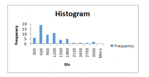
Bin	Frequency
100-300	6
301-600	19
601-900	9
901-1200	11
1201-1500	4
1501-1800	5
1801-2100	1
2100-1800	1
2400-2700	1
2700-3000	3

1. Using (a), construct a histogram.
2. Mean, median and mode

Mean	954.3667
Median	715
Mode	401

 

Question 2

1. Is above a population or a sample? Explain the difference.

The above data presented in the context of the sample instead of population because information clearly shows that it is 7 weeks data. The term sample refers to a group of members of population selected for participants in the research study. Beside of this, population indicates to select all elements possessing with common features. It includes the each and every unit in the study (Ayyub & McCuen, 2016).

1. Calculate the standard deviation of the weekly attendance. Show your workings.

 

Weeks	Weekly attendance
1	472
2	413
3	503
4	612
5	399
6	538
7	455
Standard deviation	74.06046436

 

 

 

1. Calculate the Inter Quartile Range (IQR) of the chocolate bars sold

 

Inter Quartile Range
Quartile 1	434
Quartile 2	472
Inter Quartile Range	38

 

 

1. Calculate the correlation coefficient.

From the calculation, it is found that the value of correlation coefficient is 0.967992639. It means that is a strong positive relationship between the both variables (Silverman, 2018).

Question 3

SUMMARY OUTPUT
Regression Statistics
Multiple R	0.967993
R Square	0.93701
Adjusted R Square	0.924412
Standard Error	224.5952
Observations	7
ANOVA
	df	SS	MS	F	Significance F
Regression	1	3751817	3751817	74.37736	0.000346
Residual	5	252215	50442.99
Total	6	4004032
	Coefficients	Standard Error	t Stat	P-value	Lower 95%	Upper 95%	Lower 95.0%	Upper 95.0%
Intercept	1628.689	605.9	2.688049	0.0434	71.1734	3186.205	71.1734	3186.205
X Variable 1	10.67723	1.238051	8.624231	0.000346	7.494724	13.85974	7.494724	13.85974

 

 

From the calculation, it is found that the value of the Coefficient of Determination is found 10.67723. It means that it is means that value is great and there is effective relationship between that data set (Mendenhall et al., 2016).

Question 4

From the data provided, it is found that there are 193 participants were selected total from the Holmes and external. In this, it is found that there is 47.66% (92/193 *100) probability that a randomly chosen player will be from Holmes OR receiving Grassroots training.

B

In the context of external recruitment, it is found that 66 participants are selected in this, it is found that 55 are interested in scientific training and 12 are in grassroots training. From the calculation, it can be calculated that there is 27.98% (54/193*100) probability that a randomly selected player will be External AND be in scientific training (Wieneke, 2015).

C

In the Holmes Hounds Big Bash League cricket team, 127 persons are selected from Holmes that are interest in scientific training and Grassroots training. The calculation depicts that there is 27.56% (35/127*100) probability that he is in scientific training.

D

From the case study and calculation, it can be said that in Holmes Hounds Big Bash League, the training is independent from recruitment. It is because there is not specific standard and regulation on the training needs. Figures are showing that selected participant can select the training selection according to its preference instead of the any assistance.

Question 5

A.

P(AIX)= p(A)*p(XIA)/ p(A)* p(XIA)+ p(BC)*p(YZIBC) (Source: Quirk, 2018).

= (0.55*0.2)/(0.55*0.2)+(0.45*0.8)

=0.11/(0.11+0.36)

= 0.11/0.47

= 0.2340

B.

P(X)= P(A)*P(X)+ P(B)*P(X)+ P(C)*P(X)+ P(C)*P(X)

= 0.55*0.2+0.3*0.35+0.1*0.6+0.1*0.9

=0.11+0.105+0.06+0.09

= 0.365

Question 6

A.

P(X≤2)=P(X=0)+P(X=1)+P(X=2)

= (0.1)⁰(0.90)⁸ + (0.1)¹(0.90)⁷ + (0.1)²(0.90)⁶

= 0.430+ (0.1*0.478) + (0.01*0.531)

= 0.430+ 0.0478 + 0.00531

=0.4831

B.

In one minute, average 4 people enter the store then the average number of customers entering every 2 minutes will be:

2*4= 8 people in every two minutes

Need to calculate:

P(X=9 l l=8)=8⁹*e^-8 /9Ị

= (134217728 * 0.000335463)/ 362880

= 45025.082/362880

=0.1241

Question 7

A.

P(x=2)

=

=

=

=2.3376

From z table, it is identified that probability p(z=2.3376) for X=2 will be 0.9904. So, for over $2 million, it will be P(x>2) = (1-p(x=2))

= 1-0.9904

= 0.0096

P(1<X<1.1)

=<

= <  <0

=p(-0.2597)

= 0.3974

Question 8

A.

For sufficiently large sample sizes (n≥30), it is considered that the distribution of the sample means is approximately normal. In this case, the sample size is 50 or more than 30 means the distribution of the sample means should be normal (Quinlan et al., 2019). But the distribution is not normal then a Z-distribution to test assistant’s research findings cannot be used.

B.

11 Investors agree for investment as their proportion will be 11/45= 0.2444

=0.2444-0.30/SQRT((0.30*0.70)/45)

= -0.0556/SQRT(0.21/45)

=-0.0556/SQRT(0.004667)

=-0.0556/0.068313

= -0.8139

From table, p value will be 0.2090.

 

 

References

Ayyub, B. M., & McCuen, R. H. (2016). Probability, statistics, and reliability for engineers and scientists. CRC press.

Mendenhall, W. M., Sincich, T. L., & Boudreau, N. S. (2016). Statistics for Engineering and the Sciences, Student Solutions Manual. Chapman and Hall/CRC.

Quinlan, C., Babin, B., Carr, J., & Griffin, M. (2019). Business research methods. South Western Cengage.

Quirk, T. J. (2018). Excel 2016 in Applied Statistics for High School Students. Springer.

Silverman, B. W. (2018). Density estimation for statistics and data analysis. Routledge.

Wieneke, B. (2015). PIV uncertainty quantification from correlation statistics. Measurement Science and Technology, 26(7), 074002.