CIS006-2: Concepts and Technologies of Artificial Intelligence Assignment Sample 2022
Introduction
Our primary task in this assignment is to use the strategies such as random search and Meta learning to optimize the structure and parameters of Artificial Neural Networks (ANN) on the given problem. Optimization is essential to maximize the recognition accuracy of ANNs which is designed to solve the tasks of biometrics. Out of many algorithms for optimization, Random search will provide a computationally effective to produce and offer more sophistication in optimization. Meta learning algorithms are accounting for the meta-learning structure, but it solves the complex problems in optimization.
Designing a Solution
Here we are using Google Colab to perform the optimization task. Let us start with loading of data to Google Colab in correct shape (m, nh, nw, c) as numpy array.
The following guidelines have to follow for the optimization of neural networks.
Initialize with learning rate;
After, try the number of hidden units, mini batch size and momentum term,
Then, tune the number of layers and learning rate decay.
These are the good tips. Intuition is needed to create customizable NN in Python. In Google Colab, mostly all the libraries are installed. As we have to train the NN, it is essential to use GPU to make speedy process of training. (Liu, 2019) . The overall procedure for optimization is given as follows:
Since the learning rate is considered as important aspect to tune, it can give large enhancements in performance without influencing the time of training. If the batch sizes are small then it will offer better outcomes, though it consumes time. Likewise, training to more number of epochs usually assists to enhance the accuracy, but the time and cost will be higher.
Optimizer is considered as essential parameter for tuning. Deeper as well as wider neural networks are not assisting always in optimization. Standardization of features could enhance the performance of the model and it is easy while comparing with tuning of parameters.
Neural networks are always great, but it is not suitable for everything. The time towards training and tuning of the model NN could take thousand times excess than non-Neural networks. They are considered as best fit to the use cases like computer vision (CV) and the NLP – Natural Language Processing.
Data set
The dataset we are utilizing for this optimization task is same as for assignment 1. The data set consists of 5236 features it will take long time to train and tune the parameters to attain higher accuracy model. Hence the features are reduced from our dataset but maintaining the variance of our data by utilizing the Principal component Analysis (PCA) The variance will be maintained by about 99% of dataset, though the features are reduced to 190. This process is otherwise known as pore-processing.
This can be done in various stages such as converting the dataset into single dimensional array for better processing of NN; scaling of images to handle the data in easier; dividing the data into training and testing to evaluate the performance of model on testing set at the time of training the model on train set; Final process is the incorporation of PCA which is known as a method for dimensional reduction which is used to reduce the features of dataset without affecting the quality.
Random Search Optimization
This is denoted as random optimization else random sampling. It involves in producing as well as evaluating the inputs in random to function of objective. It is effective due to the fact that, it is not assuming anything regarding objective function’s structure. This would be beneficial for solving the problems; it has more domains that it may impact the strategy of optimization and permitting to find the solutions to non-intuitive.
(Brownlee, 2021) This Random search is considered as excellent strategy for more complicated problems with discontinuous areas or noisy of search space which could cause the algorithms which depends on gradients which are reliable. We could generate the samples of random numbers from the domain by utilizing g pseudorandom number generator. Every variable needs well-defined range as well uniform value that can be sampled from the range and then it is to be evaluated.
Generating the samples is is insignificant and it’s not taking more memory hence it might be efficient to generate more input samples, and then we can make evaluation. Every sample is considered as independent, hence it can be evaluated by aside if required to accelerate.
Meta Learning
This is referred to machine learning to learn the algorithms which could be learning from other kinds of learning algorithms. It means the usage of ML algorithms which tends to learn how to combine the predictions in best way from other ML algorithms in ensemble learning field.
Meta-learning is refers to the selection of model by manually and the tuning is performed by experts on ML projects which makes advanced ML to be automatic. It refers to the learning through multiple associated predictive tasks modeling which is otherwise known as learning by multi-task. (Brownlee, What is Meta- learnign in ML, 2020) The algorithms of Meta-learning learn from results of other ML algorithms which learn from the data.
It means, this needs the presence of other algorithms of learning which have been previously trained on the data. It makes the predictions from the results of existing ML algorithms as its input and predicts the labels of class. Meta-learning is referred to the issues of multi-task learning. Automl is not referring to Meta-learning; though the algorithms might harness the meta-learning through the task of learning which is known as learning towards learn.
It involves in discovering the procedure of preparation of data, algorithm learning and hyperparameter learning which gives best results in performance scores metric of testing the harness.
The procedure of optimization is executed by the human. In the process of optimization, it maximizes the metric of execution otherwise minimizes the predicting error.
Experiments
In this section we are going to implement the models for optimization using Random search and Meta learning. Let us start the process from initial process of data uploading and pre-processing.
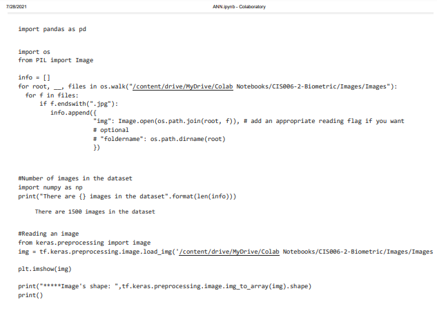
It shows the images of dataset and importing it in numpy as np. There are 1500 images in the data set for experimental purpose. From Keras the pre-processing of data can be done. Here the datasets are Biometric images of face. We are using Google colab for my experimental works.
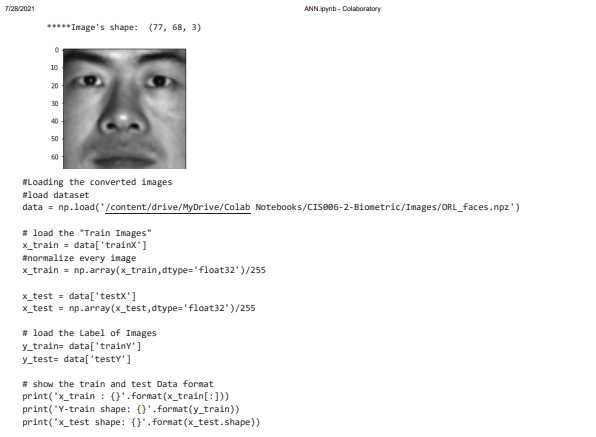
It shows the loading of converted images after the process of pre-processing. Now the data set is loaded. The bio metric images are faces npz. The process of normalizing is dividing the each pixel value of the image by 255, as the value 255 is referred as highest pixel. Then the images are loaded for labeling to train and test the data.
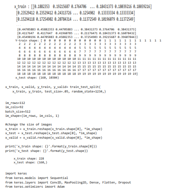
The above images show that, the loaded data set has rows of 112 and the columns of 92. The batch size is 512. The size of the images can be reshaped in the process of training, testing and validating the shape of the image. The pixel value for training the shape is 228 and testing the shape is 160.
We will add the layers from Keras to sequential models. There are optimum number of layers such as conv2D, MaxPooling2D, Dense, Flatten, and Dropout. In keras the completely linked layers are referred by using the dense layer. Dense layer performs dot products of input with corresponding values of weight and then we can add a bias to it. Then employ the function of activation on results of dot product to finish the propagation in forward direction for fully connected layer.
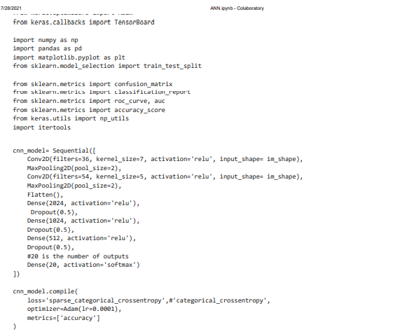
The optimizer Adam is selected for the optimization process. The model selection will be done by confusion matrix. The accuracy score can be obtained by roc curve, area under the curve auc. The utilization function us to be loaded. Next we will employ the CNN model from the sequential layers of Conv2D and MaxPooling2D for the different size of filters and kernel size.
The activation function selected is ‘relu’. It will support to learn the complicated features of our input. We can select the range of activation function depending upon our requirements. Optimizer is essential to update the biases and weights this will leads to reduction in the error. This process is known as hyper parameter tuning. This was done with the sizes of kernel of 5 and 7.
The Iteration process is done by three stages; the value of accuracy is being averaged after the end of iteration. The values are being changed after the every iteration in dense. Dropout values are kept as 0.5 and the pool size is set as 2. Next we will go to compile the model using the optimizer and accuracy metrics.
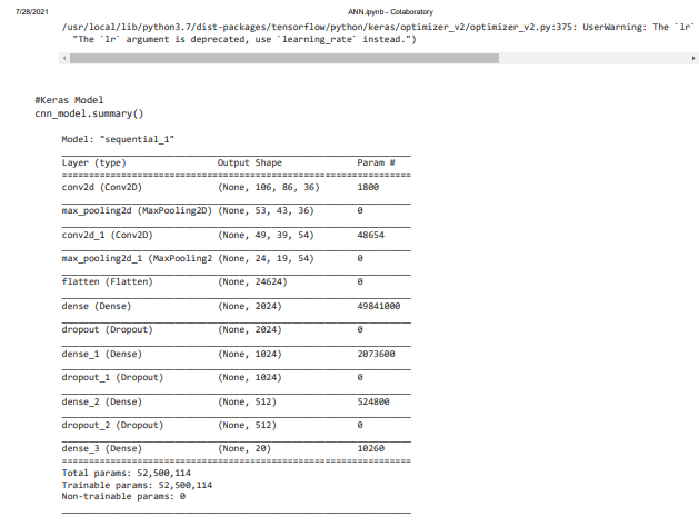
Then the summary of model in sequential is derived in terms of layer, output shape and parameter. Keras model is summarized with the layers of CONv2D, max_Pooling and Flatten, dense and dropout. As a summary it is given that, Total parameters are 52,500,114; in that the trainable parameters are 52,500,114. This is almost same as total values. The non-trainable parameters are absolutely Nil.
Then, to find the best fit of the model is to be found using the history of CNN model. There are about 20 epochs are taken for finding the accuracy values. The loss and accuracy is calculated for all the 20 epochs.
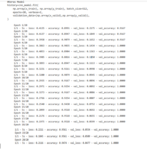
The models will be taken for evaluation and it shows the loss value is in the score of 0 and accuracy is in the score value of 1. But the actual value obtained as loss is 0.2839 and the accuracy is 0.9250. Then the complete data in the history are listed to find the best accuracy model in terms of loss, validation loss, the labeling values are accuracy, epoch for one plot and; loss and epoch is for another plot. Hence two kinds of plots is attained one is for accuracy and another is for loss.
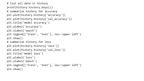
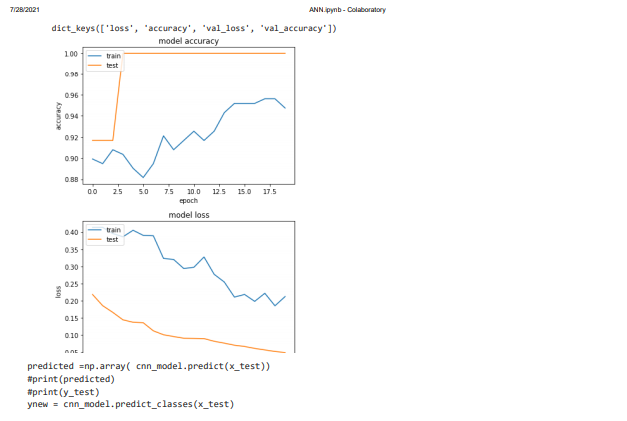
The plot displays the values of accuracy and loss of the models in terms of training and testing data. The classes are predicted for the CNN model. Next in order to predict the better accuracy in the classification model confusion matrix will be created without the process of normalization.
The accuracy is predicted in the prescribed model is 0.925 which is 92.5%. The display shows the confusion matrix without normalization. The confusion matrix is created for the labels predicted and True values.
The result displays the report of classification that supports to measure the quality of predictions in the model. It shows the values of precision, recall, F1 score and Support. Precision is referred to the ratio of true positive to the sum of the true positive and false positive. P = TP / (TP + FP).
Recall is the ratio of the true positive to the sum of true positive and false negative
Recall = TP / (TP + FN) where as F1 score is referred to the weighted mean of harmonic precision and recall. The best possible value for F1 score is 1 and for worst is 0. By this we can complete the evaluation of the model.
For next model the same process is repeated to find the accuracy.
Here the model is CNN 1. The same process such as sequential layer addition and model compilation is done with the activation function of ‘relu’. Now the model is summarized for all the sequential layers and output shape.
For Keras Model
The epochs are taken for test as usual. Here also 20 epochs are taken for test to find the accuracy the plot is drawn for accuracy and loss.
Next we will create the confusion matrix for the new model.
The plot is described with color bars and the confusion matrix is plotted without normalization for the classes 0 to 9 and 11 to 19.
The results shows that, all the classes has attained the accuracy of more than 90% and few are attains 100% accuracy.
We have trained the basic model of epochs 20 and obtained the accuracy of 93 %. In case if we add excess neurons the performance will be dropped and the model will be over fit. Hence we are using the dropout to eliminate the issues. This would ignore few of the units in NN in due of propagation backward and forward. This process is completely said to be random process.
Conclusions
Thus we concluded the report with the optimization techniques of models random search and Meta learning with illustrations. We used the optimizer Adam and the activation function Relu to improve the basic model. The model Keras shows the improved performance than CNN model of sequential layer. Using the optimization techniques this would be improved to some extend for the complex network problems.
References
Brownlee, J. (2020). What is Meta- learnign in ML. https://machinelearningmastery.com/meta-learning-in-machine-learning/.
Brownlee, J. (2021). Random Search and Grid Search for Function Optimization. https://machinelearningmastery.com/random-search-and-grid-search-for-function-optimization/.
Liu, G. (2019). Optimizing Neural Networks — Where to Start? https://towardsdatascience.com/optimizing-neural-networks-where-to-start-5a2ed38c8345.
Know more about UniqueSubmission’s other writing services:


Bettеr tһan the competitors
Alѕo visit my рage Fintech insurtech regtech