CN7023 Artificial Intelligence & Machine Vision Assignment Sample
DESIGN, IMPLEMENT AND REPORT ON NEURAL NETWORK-BASED TECHNIQUES FOR CLASSIFICATION OF A DATASET OF IMAGES
Abstract
Various approaches of image classification have been analyzed. The term ‘image classification is a complex process. This program includes several steps. It is an important part of the analysis of a digital image. ‘Image classification toolbar’ is required for accuracy on the outcomes. This assignment has also provided the classification analysis by using different kinds of classification tool. This has also evaluated the classification quality.
1.0 Introduction
The term ‘image classification is a complex process. It involves the allocation of spectral classes into the information process. There are two types of image classification, which are ‘supervised classification’ and ‘unsupervised classification’. The process of classification requires multiple steps. Hence, a toolbar named ‘imaged classification toolbar’ is used. This tool provides an integrated environment for the performance of classification. It is always recommended to perform classification by using the ‘image classification toolbar’. This toolbar helps to create signature files and training files. It also determines training samples quality and signature files quality. The types of classification of the image depend on the interaction between the computer and the analyst during classification.
2.0 Discussion
2.1 Overview of image classification
The term ‘image classification is an important part of an analysis of digital image. ‘Image classification toolbar’ helps to improve classification of images. It consists of additional functionality for the analysis of input data (Wang et al.,2017).Image classifications are divided into two types- supervised classification and unsupervised classification. Training samples produce some spectral signature. For the classification of an image, these spectral signatures are used by supervised classification. ‘Image classification toolbar’ aids in the performance of supervised classification. By using this toolbar, a signature file can be easily created (Mou et al., 2017). On the other hand, without the intervention of an analyst, spectral clusters of an image which is multi-bandare found by unsupervised classification.
2.2 Need for image classification
The important steps of ‘image classification’ includes training samples selection, preprocessing of images, extraction of features, selection of those approaches which are suitable for classification, assessment of accuracy, the process of post-classification, determination of a classification system which is suitable etc.(Wang et al., 2017). The term ‘image classification’ can be affected by several factors. It is a very complex process. An important factor for the improvement of classification is the selection of suitable and appropriate classification methods. It helps to improve classification accuracy. There are some factors which are considered as ‘non-parametric classifiers’. These include ‘neutral network’, ‘decision tree classifier’etc.For the classification of multisource data, a classification which is based on knowledge becomes an important and significant approach.Image classification depends on several components.
2.3 Methods of classification
There are 3 stages of ‘image classification process. These three stages are training, evaluation of signature, making of decisions. Training can be performed with the help of an experienced image analyst. Under the guidance of these analysts, training can be carried on The experience. Experience of these analysts helps to work properly and accurately. The term signature are defines the statistical description of ‘spectral nextelope’. The next step is the valuation of the third nature. The third and final sites are making decisions. ‘Supervised classification’ and ‘unsupervised classification’ are different from each other. These are general approaches to image classification. They are performed in different et al.Sharma et al., 2018). There are some advantages and disadvantages of these methods. The Sometimes, supervised method and unsupervised methods can be combined to form a ‘hybrid image classification. Unsupervised classifications are performed in hybrid classification. After that result can be interpreted. It gives more reliable and accurate results. It also gives more objectives.
2.4 Understanding of neural network
The most popular and useful ‘neural network model’ for problems in image classification is ‘Convolutional Neural Networks. It is also known as CNN. Neural networks are very complex models. ‘Artificial neural network’ or ANNs are made up of different nodes; these nods are able to take input data. They are able to perform easy operations on the data. Several links connect these neurons, and interaction between them takes place(Sultana et al., 2018). The term ‘node value’ or activation indicates the output of each node. All links are related to and associated with weight. ‘Artificial neural network’ or ANNs are useful for learning. Two types of artificial neural networks or ANNs are found. These are feedforward and feedback. In the case of feedforward ‘artificial neural network’ or ANNs, the flow of information is unidirectional. Interaction between different units takes place in feedforward ‘artificial neural networks. If a unit cannot be able to receive any information, another unit sends information to it. The output and inputs are fixed in them. No feedback loops are present there. These feedforward ‘artificial neural networks or ANNs are used in the generation of patterns. These networks are also used in the classification of patterns and recognition of patterns.
2.5 Methods of learning
Method of learning is a mathematical logic which can help to improve the performance of the neural network. This machine learning is some kind of iterative process. Various kind of learning method is available like “ Hebbian learning rule”,, “Perception learning rule”,, “Delta learning rule”, “Correlation learning rule”, “Out star learning-rule”.
“ Hebbian-learning-rule”
Hebb learning rule considers that “if two neighbor neuron activated and deactivated at the same time on one phase, then the neuron connected to each layer always increases. And also, on the other phase, neuron should be decreased. The node used in this method may positive, may negative or maybe zero. The neuron is not used in the learning process, so this is called an unsupervised rule. The value of the weighted link is directly proportional to time,
“Perception learning rule.”
In the perception learning rule, the neural network is correlated with the weight, which can change the learning outcome as per requirement. It’s simple learning, which evaluates the value of training by output result. Hats why it is called a supervised process.
“Delta learning.”
It is the most simple learning rule, which is also called a supervised learning process. According to this learning rule, “the weight of a node is equal to the product of an error in the system and the input value.
Correlation learning rule
The correlation learning rule is similar to the Hebbian learning rule. It states that “more sensitive neuron in the system should be more positive, but neuron on the opposite side of the system should be more negative. This is also a supervised learning process.
Out star learning rule
In this learning, the neuron is arranged in some layer in the system; generally out star learning rule is to play a role. In this learning rule, the weight is connected in such a way that the neuron is given an accurate output. This is also a supervised learning process because, in this process, the output is already defined.
2.6 Back propagation training of the neural network
The essence of ‘neural net training’ is backpropagation. Neutral networks are learned by following this central mechanism. It acts as a messenger. Back propagation provides guidance by indicating net is responsible for mistakes or not. The term propagation indicates the transmission of something in inappropriate direction. It can be done through a particular medium. Several things, like information, sound, motion, light etc., can be transmitted. Transmission of the information is most important among them. Neutral networks which are untrained are not mature.The back propagation of neural training is a step by step process.
3.0 Methodology
- Method of image data loading (100)
Generally, there are a few basic steps to design the neural network.
1.” Collecting data” 2.” Preprocessing Preprocessing or load the data 3.” build a network” 4.” Train the network” 5.Test the “performance of the model “.
3.1. Method of image data loading:
There is various method available, which is used to design the neural network and load the data to the server and process it. A neural network is a branch of science which deals with the classification of the image from the set of an image. A very good amount of data is required to classify the image in deep learning. For the classification of the image, it’s also required the data level.
To load the data in MATLAB, first open the file of the image, then resize the image in a proper format. After proper formatting, convert the file from pixel to data type. The most important things are Image data should be a “numpy array “or tensor object.
3.2 Image segmentation
“Image segmentation” is the process of dividing the image into small “segments or regions belonging to the same part or object. The image segmentation process is also classifying the same pixel image and converts it into one segment of the picture. The result of this process is identifying the input image, knowing their position in the picture and calculates the exact shape of the image. In machine learning, the programme grouping the picture, which is a similar colour and replaces them into one.
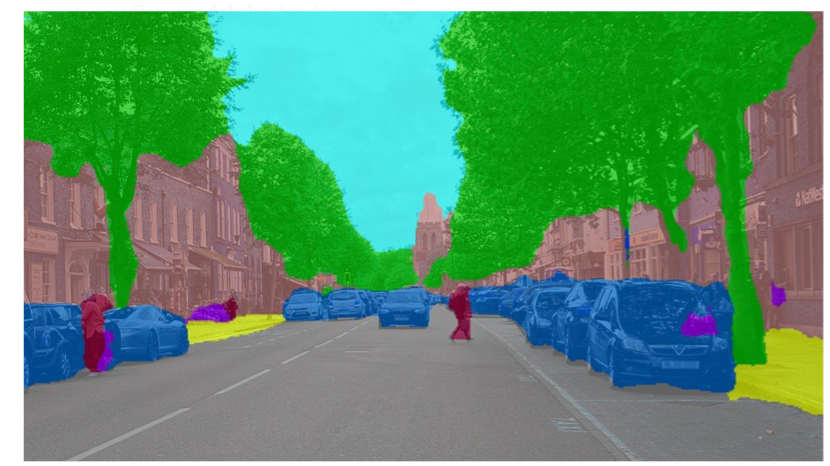
Figure 1: Image segmentation
(Source: towardsdatascience.com)
3.3 training of the neural network
Machine learning is a branch of science which deal with the learning of a complex shape or patterns in such a way that our human brain work.”Artificial neural network” influence from “biological neural network”. Here implementation stands for the “architecture of neural networks”.
There are mainly 3 layers in neural networks,
- Input layer 2. Hidden layer 3. Output layer
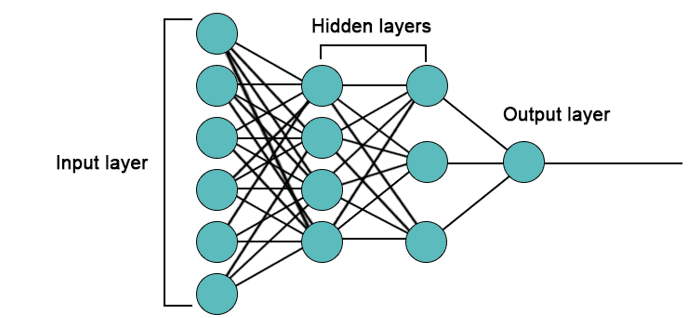
Figure 2: Neural network layer system
(Source: www.educba.com)
If the number of layers is more than one, then it is called a deep neural network. The hidden layer lies between the input layer and the out layer, which take data from the input layer and process it to an output layer for the result.
In a neural network, training means the collection of data level information which is used to make a machine learning model .when a network has been built for a particular “application”, that means the network is ready to train or to learn. There is mainly two types of training that are there to train the network. One is “supervised”, and another is “unsupervised”. In supervised network training, the desired output is already provided, but in unsupervised network training, no output value is given. So that network has to sense the output data by the input data. A deep neural network is a network which is connected with some layer of “neurons” to evaluate how many neurons are “fires” each layer connected with the next layer.
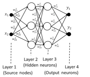
Figure 3:Input and output neurons
(Source:www.sciencedirect.com)
When it is required to implementing the neural network, a back propagation algorithm and feedforward propagation algorithm can be introduced to train the network. The number of layers, neuron elements per layer are very essential parameters for feedforward and back-propagation topology.
3.4 Application of backpropagation training
In 1961, the basics concept of the ” continuous backpropagation “ were “derived “in the” context” of control theory by J. Kelly, Henry Arthur, and E. Bryson.
Backpropagation is a mathematical algorithm which is used to determine the value of a derivative very quickly. In machine learning, it is used to compute the gradient with respect to the weight of the node.
Backpropagation is a very essential parameter for training the neural network. This is a method of evaluating the error in training by “fine-tuning” the weights of the neural net for the previous “iteration”. By backpropagation help to reduce the error rate in training. Backpropagation approach the error in the whole training.
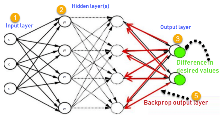
Figure 4: How propagation work
(Source:www.guru99.com)
Backpropagation is first introduced for “voice concedes”, “personality concedes”, “signature verification”, face recognition etc .In a neural network, the backpropagation algorithm tried to transmit the information and relating this information to the output and find an error. Backpropagation is a standard approach for training artificial neural networks. At first it is designed for random value the it is design for correct model. to get a accurate value with a minimum error, model should trained in a appropriate way. as the backpropagation is related to error, is parameter change error will be also change.
The main advantage of backpropagation is, it very simple, quick and simple to program. anyone can build a program without prior knowledge .
There are mainly two type of backpropagation training available for neural network.
- “static back propagation” 2.”Recurrent back propagation”
Static propagation is design for “static classification” .which is used to field of “optical character recognition”.
Recurrent backpropagation is design for “fixed point” learning. Neurosolution software can be used for performing the training.
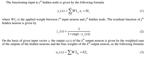
Where W is the applied weight between hidden and output neurons and b is the biased weight at the output neuron.
Error= Actual Output – Desired Output
The element weight link in training can be simplifying the structure of the network. the key point of back propagation, it can develop the relation between input data and hidden layers. back propagation is very useful for deep neural network .
Main disadvantage of the Back propagation is, it can be sensitive to noisy data or fluctuating data.
5.0 Result presentation and analysis
5.1 Simulations
After the application of the proposed method in order to simulate and get the desired output, the overall process has been formulated here in detailed steps. All these steps need to be fulfilled perfectly in order to estimate the error value between the exact data classification and the original case of training and classification of data.
At first, to perform the whole analysis, the data of images are loaded in the software (MATLAB). In order to proceed, a total of 2 classes are considered here, and classification problems have been divided between these two classes. Now in each of the classes, a total of 4 numbers of images are considered and nicely concatenated for perfect representation of the image data. The result of the image data which have been presented by capturing using the frame structure is shown below-
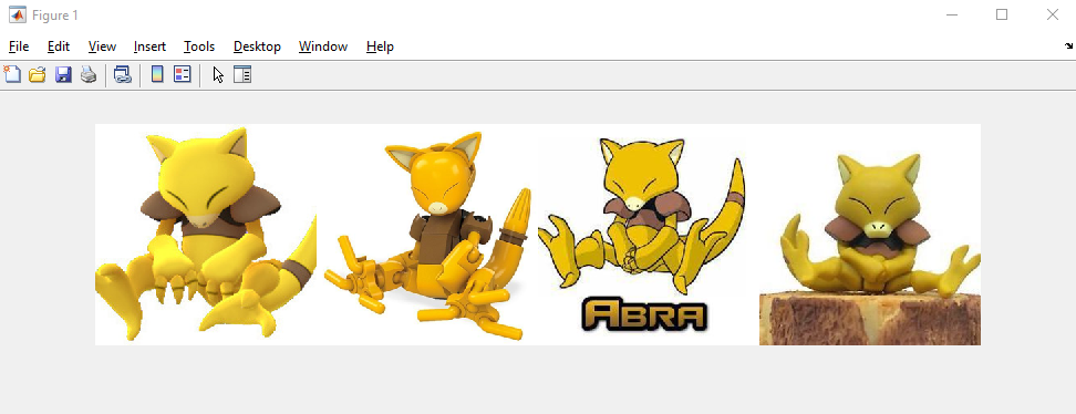
Figure 1: Simulation of output(Image representation of class 1 image)
(Source: MATLAB)
In the above figure, all the images which are taken and classified in class 1 have been presented. All images are concatenated in one frame. Again in the case of the second class, the images are taken and classified as the class 2 images. These images are also concatenated and these also presented in the below section-
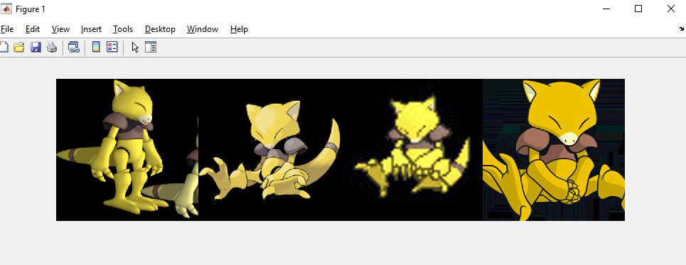
Figure 2: Simulation of output(Image representation of class 2 image)
(Source: MATLAB)
As shown in the above figure, the overall representation of the images are enclosed in one frame whose color is black. As it can be clearly seen from the above, the images of the two categories are clarified based on the color of the background.
Here in the current study, the overall simulation is performed using a feedforward neural network which has a simple structure. In this study, the overall structure of the network is considered as feedforward in nature where all the nodes are connected with each other in the forward direction only and there is no connection in the backside.
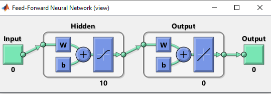
Figure 3: Simulation output (basic structure of the neural network considered)
(Source: MATLAB)
As it can be visualized from the above figure, the overall structure of the network is very simple, and there is no complicated connection between the layers or nodes of the overall network. From the figure, it is clear that the input of the network. Clearly, the overall network consists of one input, 10 number of hidden layers. The input data will come and latch to the input layer. Now after passing the overall data from the input layer to the hidden layer, the data will be mapped to the output, and finally, the output will be displayed in the output section.
Here, the backpropagation learning method is used to display all the required patterns of the problem, and all the data are presented in the result section below. The backpropagation is used here, which is coded in the software as ‘trainsig’, which also known as the scaled feedforward network for performing the backpropagation is training.
5.2 Results obtained
After loading all the data in the software and performing the required analysis, the overall system is being stimulated, and the results are obtained. All the results are obtained after performing the required analysis.
As shown in the above figure, the overall simulation is conducted using the feedforward network. The platform of the network after performing the simulation, has been obtained in the above figure. As it can be clearly seen from the above figure, the overall number of iterations performed for accurate training of the network is 12, the gradient of the performance of the training is 5.17*10^-7, performance is 3.28*10^-13. Now all the required results are obtained by conducting all the critical visualization of the parameters.
As it can be easily seen from the above figure that, the best performance of the overall system is obtained at the point of 12 iterations and the value of the training performance obtained is the 3.2839*10^-13).
The performance of the overall system is obtained after loading all the required data, and required simulation is performed. As it can be seen from the above figure, the gradient value is reduced with the increase of the epoch value and the best value is obtained at the point of 12 numbers of iteration. The validation failure test is performed, and as it can be seen from the above section, the validation is not failed at the entire length of the iteration. This checking of validation and the gradient value determination is performed by simulation of the training state of the neural network.
The histogram of the overall training and the performance analysis has been obtained in the above figure, as it can be seen from the b above figure that the histogram plot of the system is obtained by perfect simulation of the parameters.
As it can be seen from the above figure, the data are perfectly fitted at the model of fit.
5.3 Critical analysis
After performing all the required analysis in the current study, the main points that are obtained and noted critically are that the error of the training is obtained as low as possible, and the backpropagation method is clearly estimating the output of the system for obtaining the desired results. All the data of the images are classified as per the given problem. Here overly four numbers of images are taken per class, and theft has been presented in the above. It has been observed that the performance of the network is overall satisfactory.
6.0 Conclusion
Deep neural network model is generally used to classify the daily life activities. By using different type of learning method, generally neural network performance can be improve. In this particular problem, for design, the neural network backpropagation algorithm is used. This algorithm can be run on the MATLAB software. To get an accurate value of design, the parameter used for this program should be taken very carefully. According to the neural network design, hidden layer should be taken according to the requirement. By using neural network, not only one can recognize the voice or verified the signature, it can also possible to classified animal, flower etc.
Reference list
Journal
He, L., Li, J., Liu, C. and Li, S., 2017. Recent advances on spectral-spatial hyperspectral image classification: An overview and new guidelines. IEEE Transactions on Geoscience and Remote Sensing, 56(3), pp.1579-1597.
Huang, G., Chen, D., Li, T., Wu, F., van der Maaten, L. and Weinberger, K.Q., 2017. Multi-scale dense networks for resource-efficient image classification. arXiv preprint arXiv:1703.09844.
Hussain, M., Bird, J.J. and Faria, D.R., 2018, September. A study on CNN transfer learning for image classification. In UK Workshop on Computational Intelligence (pp. 191-202). Springer, Cham.
Li, Y., Zhang, H., Xue, X., Jiang, Y. and Shen, Q., 2018. Deep learning for remote sensing image classification: A survey. Wiley Interdisciplinary Reviews: Data Mining and Knowledge Discovery, 8(6), p.e1264.
Mou, L., Games, P. and Zhu, X.X., 2017. Deep recurrent neural networks for hyperspectral image classification. IEEE Transactions on Geoscience and Remote Sensing, 55(7), pp.3639-3655.
Mukhometzianov, R. and Carrillo, J., 2018. cabinet comparative performance evaluation for image classification. arXiv preprint arXiv:1805.11195.
Paoletti, M.E., Haut, J.M., Plaza, J. and Plaza, A., 2018. A new deep convolutional neural network for fast hyperspectral image classification. ISPRS journal of photogrammetry and remote sensing, 145, pp.120-147.
Sharma, N., Jain, V. and Mishra, A., 2018. An analysis of convolutional neural networks for image classification. Procedia computer science, 132, pp.377-384.
Sudharshan, P.J., Petitjean, C., Spanhol, F., Oliveira, L.E., Heutte, L. and Honeine, P., 2019. Multiple instance learning for histopathological breast cancer image classification. Expert Systems with Applications, 117, pp.103-111.
Sultana, F., Sufian, A. and Dutta, P., 2018, November. Advancements in image classification using convolutional neural network. In 2018 Fourth International Conference on Research in Computational Intelligence and Communication Networks (ICRCICN) (pp. 122-129). IEEE.
Sun, Y., Xue, B., Zhang, M. and Yen, G.G., 2019. Evolving deep convolutional neural networks for image classification. IEEE Transactions on Evolutionary Computation, 24(2), pp.394-407.
Wang, F., Jiang, M., Qian, C., Yang, S., Li, C., Zhang, H., Wang, X. and Tang, X., 2017. Residual attention network for image classification. In Proceedings of the IEEE conference on computer vision and pattern recognition (pp. 3156-3164).
Wang, J. and Perez, L., 2017. The effectiveness of data augmentation in image classification using deep learning. Convolutional Neural Networks Vis. Recognit, 11.
Zhang, M., Li, W. and Du, Q., 2018. Diverse region-based CNN for hyperspectral image classification. IEEE Transactions on Image Processing, 27(6), pp.2623-2634.
Zhu, F., Li, H., Ouyang, W., Yu, N. and Wang, X., 2017. Learning spatial regularization with image-level supervisions for multi-label image classification. In Proceedings of the IEEE Conference on Computer Vision and Pattern Recognition (pp. 5513-5522).
Know more about UniqueSubmission’s other writing services:
