Financial Modeling Coursework 2020

a)      Quarterly GDP Data for Austria

In the view of Jenkins (2006), the autoregressive integrated moving average (ARIMA) model is one of the important model classes that are used to describe s single time series. The assignment chooses this model to analyze the time series secondary data of a country. For this purpose, the assignment chooses Austria; an OECD nation and collect the quarterly GDP data for the last fifty years i.e. 1963 – 2013. The assignment uses STATA software as a base to perform time series test and graphical analysis in order to predict the quarterly GDP of Austria for the coming 50 years.

b)     Time Series Plot

In Stata, simple time series command is used to plot the trend line of Austria’s quarterly GDP over the last 50 years. The graph below provides the trend line of quarterly GDP rates as change over the same quarter and analysis shows downward GDP movement during the economic crisis of 2007-2009.

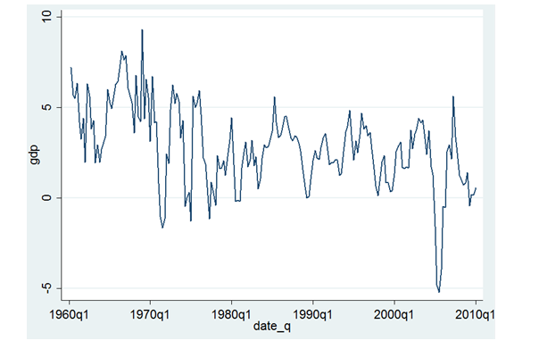
Graph 1: Quarterly GDP Growth Rates of Austria

(Source: OECD, 2015)

A look at the graph below, however, depicts an upward movement with slight variations during the crisis period. The graph below depicts a rather sharp trend of GDP.

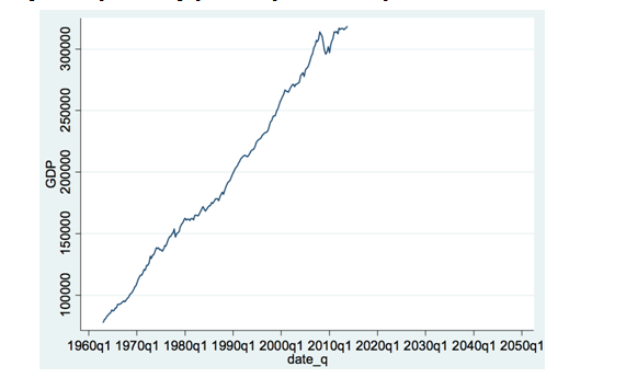
Graph 2: Quarterly GDP Trend

For better understanding, log function is used on the GDP data; the graph below shows that Austrian economy’s connection with the European Union State members had significant affect on the GDP performance of the country. As a consequence of 2007-08 crises, Austrian GDP reported variations in the late 2009; however, the graph below depicts a visible recovery of Austrian economy due to subsidized government projects. Nonetheless, time series analysis shows that the GDP trend is non-stationary and non-static over the given time period.

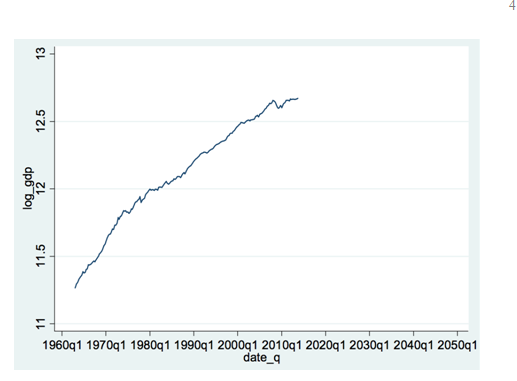
Graph 3: Trend of Log_GDP

c)      Autocorrelation Function (ACF) and the Order of AR and MA

In the Dickey-Fuller test, if test statistic is greater than all the values at three different critical levels then the null hypothesis can be rejected. Stata results in the figure below depict an opposite situation as the test statistics value is -0.175 and it is small than the three critical values i.e. -3.476 at 1%, -2.883 at 5% and -2.573 at 10%. In other words, Dickey-Fuller unit root test indicates that the null hypothesis of GDP series cannot be rejected.

The above illustration provides an indication for the presence of unit root problem, which is solved through the first differential (See figure below). For this purpose, Dickey-Fuller test is re-performed with the first differential; this turns the non-stationary GDP series into a stationary series. The figure below shows that test statistics value is smaller than all the three critical values; hence, the series is stationary.

The auto-correlation graph (Ac) below provides evidence for the presence of higher lag in the data.

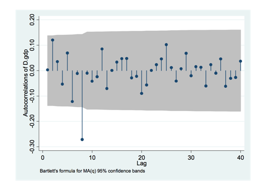
Graph 4: AC

        i.            Partial Autocorrelation Function (PACF) Plot

In line with Ac results, the Pac plot below also depicts higher lags, which means that the stationary series achieved through first differential above is providing insignificant values.

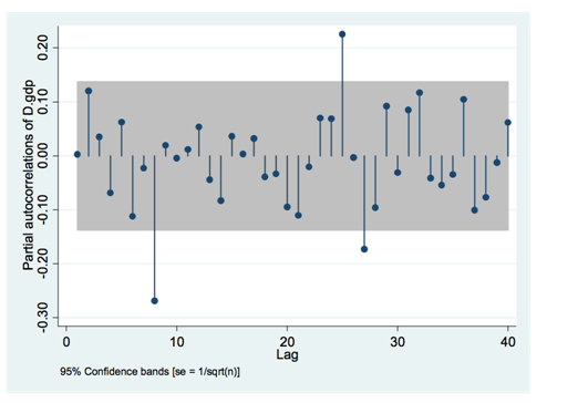
Graph 5: Pac

In order to choose the right type of ARIMA model, log_gdp command is performed in the Stata software. As can be seen in the figure below, z(t) value is lower than the standard value i.e. 0.05; this means that the series is stationary and the model selected for evaluation is Arima model with D=0.

The choice of model can be justified through Ac and Pac plots below, for example, the Ac graph below depicts gradual decline. Analysis shows significant values till the 16^th lag and these are certainly different from zero.

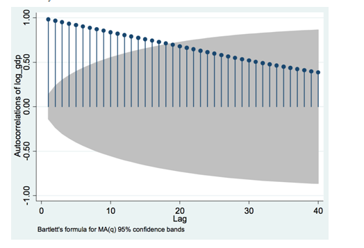
Graph 6: Autocorrelation

The Pac graph below provides clear evidence of partial coefficient at points such as lag 1 and 9; thus, values at these lag points are significant and outside the 95% confidence interval. In contrast, other lags report insignificant values; hence, p-value for Arima model is suggested to be 1.

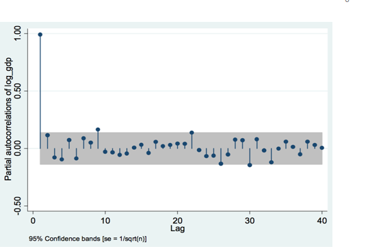
Graph 7: Partial Autocorrelation

d)     Type of ARIMA Model and Rationale

Since the above testing provides one significant point in Pac plot and declining trend of Ac, the proposed ARIMA(p,d,q) is ARIMA(1,0,0). Normally, appropriate model is done through the AIC or BIC testing (Tsay, 2010); however, in the present context, the thumb rule of selecting the model with the lowest value may not be applicable. Keeping this into consideration, ARIMA(1,0,0) with Dickey-Fuller with log is selected as the appropriate model type because the above tests depict only one model i.e. ARIMA(1,0,0).

e)      Forecasting the GDP Growth

In the Stata, following commands are used to create a forecast the GDP of Austria over the next fifty years.

As illustrated in the graph below, Austrian GDP is expected to remain flat and stable in the coming fifty years; hence, the trend is plotted as a straight line. Since the model intends to study the effect of financial crisis on the forecast, ARIMA 2007 model is applied. The graph below forecasts the GDP trend with the influence of crisis.

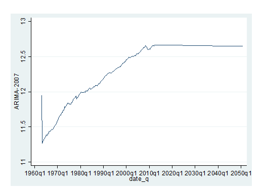
Graph 8: ARIMA 2007

According to analysis, Austria’s GDP remained under the sharp influence of economic crisis; evidence to the notion can be taken from the sharp GDP decline from 12.62% (2007) to 0.02% (2008).

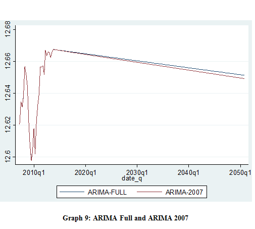
Graph 9: ARIMA Full and ARIMA 2007

In the graph above, ARIMA FULL line moves above the ARIMA 2007 line; since ARIMA FULL values are higher than ARIMA 2007; the evaluation suggests that unlike ARIMA 2007, ARIMA FULL line indicates no impact of financial crisis on Austria’s GDP.

f)       The Monte-Carlo Experiment

Following are the commands to prove the statement that Dickey-Fuller model may not be suitable for stationary series if the model is based on time trend.

At x=0, the p-vale is 95.8%, which means the Dickey-Fuller test with no trend is more reliable than otherwise. The figure below indicates that the Dickey-Fuller value at x=1 is significant; however, p-value is only significant for 4.2% of the total 1000 frequency. Hence, in case of trend model, Dickey-Fuller is less suitable.

On a simple note, the evaluation suggests that the Dickey-Fuller test with trend model is less suitable for stationary test and it cannot be relied as the results are very weak.

References

Jenkins, M. G. (2006). Autoregressive–Integrated Moving Average (ARIMA) Models, in Encyclopedia of Statistical Sciences, 1-6.

OECD. (2015). Quarterly National Accounts. [online] Available from <https://stats.oecd.org/index.aspx?queryid=350#> [28^th April 15]

Tsay, S. R. (2010). Analysis of Financial Time Series. New Jersey: John Wiley & Sons.