Advanced Topics in Artificial Intelligence Assignment 2020

 Overview

This paper plots a first stage in the advancement of a multi-strategy flaw finding framework to encourage the on-line observing of a modern siphoning framework, which in time it is trusted will permit on-condition (essential instead of safeguard) upkeep.

A point by point reenactment model of the framework is introduced, alongside a disentangled straight portrayal for use in the demonstrative calculations.

Two unique ways to deal with model-based shortcoming identification are illustrated, in view of spectators and parameter estimation. The initial phase in consolidating these strategies is talked about and the increases that can be accomplished utilizing a mix of various techniques are illustrated.

On condition upkeep, as the name proposes, is an approach whereby support is possibly done when the state of the plant warrants it, as opposed to at standard, pre-decided interims.

To execute this kind of arrangement, the plant administrators must be certain that the condition of the plant can be resolved with a sensible level of exactness.

Techniques, for example, vibration checking joined with administrator information and experience have up to this point been the premise of the upkeep architects’ tool stash.

Such techniques give a method for identifying mechanical issues, for example, wear. In any case, their capacity to identify pressure driven issues, for example, spillage is constrained.

The strategy for breaking down vibration results for changes in the pattern of, state, the sufficiency at certain key frequencies, likewise has the disservice of any edge based technique – the issue might be recognized when it has arrived at a specific level of seriousness.

Constant speed testing

load PumpCharacteristicsData Q0 H0 M0 % manufacturer supplied data for pump’s delivery head

figure

plot(Q0, H0, ‘–‘);

xlabel(‘Discharge Rate Q (m^3/h)’)

ylabel(‘Pump Head (m)’)

title(‘Pump Delivery Head Characteristics at 2900 RPM’)

grid on

legend(‘Healthy pump’)

load PumpCharacteristicsData Q1 H1 M1  % signals measured for a pump with a large clearance gaphold onplot(Q1, H1);   load PumpCharacteristicsData Q2 H2 M2  % signals measured for a pump with a small clearance gapplot(Q2, H2);  legend(‘Healthy pump’,’Large clearance’,’Small clearance’)hold off

Preliminary analysis

w = 2900; % RPM% Healthy pump[hnn_0, hnv_0, hvv_0, k0_0, k1_0, k2_0] = linearFit(0, {w, Q0, H0, M0});% Pump with large clearance[hnn_1, hnv_1, hvv_1, k0_1, k1_1, k2_1] = linearFit(0, {w, Q1, H1, M1});% Pump with small clearance[hnn_2, hnv_2, hvv_2, k0_2, k1_2, k2_2] = linearFit(0, {w, Q2, H2, M2});X = [hnn_0 hnn_1 hnn_2; hnv_0  hnv_1  hnv_2; hvv_0  hvv_1  hvv_2]’;disp(array2table(X,’VariableNames’,{‘hnn’,’hnv’,’hvv’},…    ‘RowNames’,{‘Healthy’,’Large Clearance’, ‘Small Clearance’}))

Y = [k0_0 k0_1 k0_2; k1_0  k1_1  k1_2; k2_0  k2_1  k2_2]’;disp(array2table(Y,’VariableNames’,{‘k0′,’k1′,’k2’},…    ‘RowNames’,{‘Healthy’,’Large Clearance’, ‘Small Clearance’}))

Involving Uncertainty

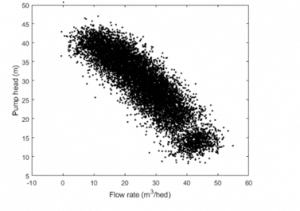
load FaultDiagnosisData HealthyEnsembleH = cellfun(@(x)x.Head,HealthyEnsemble,’uni’,0);Q = cellfun(@(x)x.Discharge,HealthyEnsemble,’uni’,0);plot(cat(2,Q{:}),cat(2,H{:}),’k.’)title(‘Pump Head Characteristics Ensemble for 5 Test Runs’)xlabel(‘Flow rate (m^3/hed)’)ylabel(‘Pump head (m)’)

Anomaly Detection

load FaultDiagnosisData HealthyEnsemble[HealthyTheta1, HealthyTheta2] = linearFit(1, HealthyEnsemble);meanTheta1 = mean(HealthyTheta1,1);meanTheta2 = mean(HealthyTheta2,1);covTheta1  = cov(HealthyTheta1);covTheta2  = cov(HealthyTheta2);% Confidence ellipsoid for pump head parametersf = figure;f.Position(3) = f.Position(3)*2;subplot(121)helperPlotConfidenceEllipsoid(meanTheta1,covTheta1,2,0.6);   xlabel(‘hnn’)ylabel(‘hnv’)zlabel(‘hvv’)title(‘2-sd Confidence Ellipsoid for Pump Head Parameters’)hold on% Confidence ellipsoid for pump torque parameterssubplot(122)helperPlotConfidenceEllipsoid(meanTheta2,covTheta2,2,0.6); xlabel(‘k0’)ylabel(‘k1’)zlabel(‘k2’)title(‘2-sd Confidence Ellipsoid for Pump Torque Parameters’)hold onload FaultDiagnosisData TestEnsemble% Test data previewdisp(TestEnsemble{1}(1:5,:)) % first 5 measurement rows from the first ensemble member

% TestTheta1: pump head parameters% TestTheta2: pump torque parameters[TestTheta1,TestTheta2] = linearFit(1, TestEnsemble);subplot(121)plot3(TestTheta1(:,1),TestTheta1(:,2),TestTheta1(:,3),’g*’)view([-42.7 10])subplot(122)plot3(TestTheta2(:,1),TestTheta2(:,2),TestTheta2(:,3),’g*’)view([-28.3 18])

Fault Isolation

load LabeledGapClearanceData HealthyEnsemble LargeGapEnsemble SmallGapEnsemble[HealthyTheta1, HealthyTheta2] = linearFit(1,HealthyEnsemble);[LargeTheta1, LargeTheta2]     = linearFit(1,LargeGapEnsemble);[SmallTheta1, SmallTheta2]     = linearFit(1,SmallGapEnsemble);helperPlotHistogram(HealthyTheta1, LargeTheta1, SmallTheta1, {‘hnn’,’hnv’,’hvv’})

helperPlotHistogram(HealthyTheta2, LargeTheta2, SmallTheta2, {‘k0′,’k1′,’k2’})

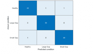
% Pump head confusion matrixfigurepumpModeLikelihoodTest(HealthyTheta1, LargeTheta1, SmallTheta1)

% Pump torque confusion matrixpumpModeLikelihoodTest(HealthyTheta2, LargeTheta2, SmallTheta2)

Fault mode’s classification

load MultipleFaultsData% Compute pump head parametersHealthyTheta = linearFit(1, HealthyEnsemble);Fault1Theta  = linearFit(1, Fault1Ensemble);Fault2Theta  = linearFit(1, Fault2Ensemble);Fault3Theta  = linearFit(1, Fault3Ensemble);Fault4Theta  = linearFit(1, Fault4Ensemble);Fault5Theta  = linearFit(1, Fault5Ensemble);Fault6Theta  = linearFit(1, Fault6Ensemble); % Generate labels for each mode of operationLabel = {‘Healthy’,’ClearanceGapWear’,’ImpellerOutletDeposit’,…    ‘ImpellerInletDeposit’,’AbrasiveWear’,’BrokenBlade’,’Cavitation’};VarNames = {‘hnn’,’hnv’,’hvv’,’Condition’};% Assemble results in a table with parameters and corresponding labels N = 50; T0 = [array2table(HealthyTheta),repmat(Label(1),[N,1])];T0.Properties.VariableNames = VarNames;T1 = [array2table(Fault1Theta), repmat(Label(2),[N,1])];T1.Properties.VariableNames = VarNames;T2 = [array2table(Fault2Theta), repmat(Label(3),[N,1])];T2.Properties.VariableNames = VarNames;T3 = [array2table(Fault3Theta), repmat(Label(4),[N,1])];T3.Properties.VariableNames = VarNames;T4 = [array2table(Fault4Theta), repmat(Label(5),[N,1])];T4.Properties.VariableNames = VarNames;T5 = [array2table(Fault5Theta), repmat(Label(6),[N,1])];T5.Properties.VariableNames = VarNames;T6 = [array2table(Fault6Theta), repmat(Label(7),[N,1])];T6.Properties.VariableNames = VarNames; % Stack all data% Use 30 out of 50 datasets for model creationTrainingData = [T0(1:30,:);T1(1:30,:);T2(1:30,:);T3(1:30,:);T4(1:30,:);T5(1:30,:);T6(1:30,:)]; % Create an ensemble Mdl of 20 decision trees for predicting the % labels using the parameter valuesrng(3) % for reproducibilityMdl = TreeBagger(20, TrainingData, ‘Condition’,…   ‘OOBPrediction’,’on’,…   ‘OOBPredictorImportance’,’on’)

% Compute out of bag errorfigureplot(oobError(Mdl))xlabel(‘Number of trees’)ylabel(‘Misclassification probability’)

ValidationData = [T0(31:50,:);T1(31:50,:);T2(31:50,:);T3(31:50,:);T4(31:50,:);T5(31:50,:);T6(31:50,:)];PredictedClass = predict(Mdl,ValidationData);E = zeros(1,7);% Healthy data misclassificationE(1) = sum(~strcmp(PredictedClass(1:20), Label{1}));% Clearance gap fault misclassificationE(2) = sum(~strcmp(PredictedClass(21:40), Label{2}));% Impeller outlet deposit fault misclassificationE(3) = sum(~strcmp(PredictedClass(41:60), Label{3}));% Impeller inlet deposit fault misclassificationE(4) = sum(~strcmp(PredictedClass(61:80), Label{4}));% Abrasive wear fault misclassificationE(5) = sum(~strcmp(PredictedClass(81:100), Label{5}));% Broken blade fault misclassificationE(6) = sum(~strcmp(PredictedClass(101:120), Label{6}));% Cavitation fault misclassificationE(7) = sum(~strcmp(PredictedClass(121:140), Label{7}));figurebar(E/20*100)xticklabels(Label)set(gca,’XTickLabelRotation’,45)ylabel(‘Misclassification (%)’)

The pumping framework whereupon this work is based comprises of 8 radiating siphons which supply water to a helper cooling circuit at a force station.

These 8 siphons work two by two, with each pair providing the water for one portion of the plant. Under typical conditions one of the siphons in each pair would be operational (obligation siphon) and the other siphon would be on reserve.

The water is drawn from the ocean through strainers to expel flotsam and jetsam, before being siphoned through to the framework. All through the framework, valves impact association of the siphons to the elective strainers and pipework.

Bibliography

Popadiuc, P., Progress Rail Locomotive Inc, 2019. Machine system having submersible pumping system, and method. U.S. Patent Application 10/240,562.

Sontake, V.C. and Kalamkar, V.R., 2016. Solar photovoltaic water pumping system-A comprehensive review. Renewable and Sustainable Energy Reviews, 59, pp.1038-1067.

Rondeau, J., Schlumberger Technology Corp, 2018. Mixing system for cementing applications. U.S. Patent 10,100,603.