
APPLICATION OF LINEAR MODELLING APPROACHES IN SEASONAL RAINFALL FORECASTING ASSIGNMENT 2020
Abstract
The present dissertation is based on the applications of linear statistical analysis for measuring the seasonal rainfall forecasting. This research aims to test the nature and pattern of the seasonal rainfall forecast, varied in different regional zone of Australia. Data is collected from the New South Wales Rainfall report of 2016-2017 and through the use of linear regression the data has been analysed.
The first chapter deals with the formulation of research objectives and questions, followed by an appropriate rationale for conducting this research. A short background of the research as well as significant information about the concerned company is also provided. The objective of this study is to identify the factors influencing seasonal rainfall and study the nature of diverse seasonal rainfall. In addition, the study is also aimed to investigate the rainfall pattern in Australian region. In the second chapter, a proper literature review is also conducted to authenticate the statement of the objectives and realize the importance of concepts of measuring rainfall data and steps related to this. The models of various esteemed and eminent scholars are taken into consideration for academic support of this research topic.

The third chapter has focused on the research methods used in the dissertation. The research has followed positivism philosophy, deductive approach and explanatory design. Secondary quantitative data collection methods have been followed through the implementation of statistical analysis of 50 rainfall station data. With the help of these data, in the fourth chapter, the researcher has acquired findings which have assisted to the researcher for achieving research objectives. The researcher, with the application of SPSS method to yield optimum and accurate results, has also conducted a proper data analysis. The findings evaluate that the team employees of the company contain a highly positive attitude towards team effectiveness. They opine that team effectiveness can enhance their performance.
The fourth chapter or the data findings have been presented in the form of tables and charts. The analysis section highlights the key implications of regression results of six different regression tests performed by regressing 6 different duration based rainfall intensities on total yearly rainfall respectively. The sequence of regression tests proceeding from first regression to sixth regression demonstrates the significance of relationship between 3 hrs of rainfall, 6 hrs of rainfall, 12 hrs of rainfall, 24 hrs of rainfall, 48 hrs of rainfall and 72 hrs of rainfall and total yearly rainfall in chosen 50 different rainfall stations of NSW region of Australia in bona fide terms. The significance obtained in regression relationship in each tests is seen to validate the regression strength in each of the two considered variables of each regression model with absolute precision.
The concluding chapter has linked the objectives with the data findings. SMART recommendations are provided. It is recommended time series based seasonal forecasting and multivariate regression analysis is needed to be done. With the implementation of these techniques, researchers can analyse better seasonal rainfall forecasting sessions in future works.
Acknowledgement
Firstly, I am thankful to my professors, who have guided me all through the research work and imposed courage to conduct the work in a proper manner. I am overwhelmed to state that without the sincere cooperation of the staff members of rainfall stations, I could have never succeeded in completing the work with complete zeal. I am thankful to my friends and fellow members for their faith in me regarding this task. Above all, I thank God to develop the will power within myself for completion of the task in a prosperous manner
The importance of econometrics forecasting to study varieties of seasonal rainfall patterns in Australia is the very important subject of study. The scope of this research is based on highlighting the adopted rationale of the study of implications of seasonal rainfall diversity on Australian environment, especially in NSW. The various facets of the study of the seasonal variance of rainfall in terms of its impact on various segments of the Australian economy are a subject of interest for weather experts in the Australian economy. This is being dealt in depth via suitable methods of the linear regression of latitudinal and longitudinal lengths of rainfall intensities on time periods respectively.
There is seen a growing interest among researchers to study trends in rainfall diversity of seasonal nature in and across the world for the sake of keeping an eye on adverse climatic conditions.This is done tackle the adversities of heavy rainfall associated harsh climatic conditions on the economy of developed economies like Australia. As per Andersen et al. 2015, p.2315), many methods are developed to study or test the impact of irregularities of rainfall pattern due to the seasonal diversity associated with it in NSW area of Australia in bona fide terms respectively. Hence to study the historical data rainfall, methods are developed via detailed research procedures undertaken by various weather and climatic experts in and around Australian economy in stringent terms and procedures.
Both predictions of intense rainfall for longer periods and lower intensity based rainfall for shorter periods can be predicted via the use of these forecasting methods.One common method especially used to study the impact of diverse or irregular seasonal rainfall in Australia is an econometrics based linear regression model based method which studies the impact of rainfall appropriately. Both the study of latitudinal and longitudinal diversities of rainfall can be performed under this process in terms of its impact over the period of years of its occurrence in Australian territory.
The aim of this research is to test the nature and pattern of seasonal rainfall variation in Australia as per the data collected from rainfall stations in NSW region of Australian economy through the use of linear regression modelling of econometric theory. The primary objective is to study the implications of rainfall based diversities in different seasonal periods of Australia on different time periods or years in Australia.
The objectives of the research are as follows:
1.To study the nature of diversity of seasonal rainfall variance in Australian region of NSW
2.To identify the pattern of diversity of seasonal rainfall in Australian region of NSW
3.To analysethe scattered variability of seasonal rainfall variance in NSW region of Australia via the use of linear regression method
4.To study the impact of the seasonal variance of rainfall on different time periods in NSW region of Australia.
The questions of the research are as follows:
1.What is the nature of diversity of seasonal rainfall variance in an Australian region of NSW?
2.What is the intensity of diverse seasonal rainfall in Australian region of NSW?
- What is the scattered variability of seasonal rainfall variance in NSW region of Australia via the use of linear regression method?
- What is tha impact of the seasonal variance of rainfall on different time periods in NSW region of Australia?
The research rationale is to test the significance of the use of linear regression analysis on the test of nature and pattern of seasonal rainfall variance in NSW region of Australia in the appropriate manner. This is performed with the sole aim of throwing light on the variance of irregularities of rainfall intensities in different seasonal periods or durations in the considered region of Australian territory in both general and specific terms respectively. As per Lawson et al. (2015, p.954), proper forecasting and prediction of the seasonal variance of data in NSW region are to be tested via regression method to throw light on the efficiency of use of the method to study the implications of irregularities of seasonal rainfall on vulnerable Australian environment in bona fide terms and perspectives(Yang and Yu, 2015, p.185).The major reason for the study of the seasonal variance in seasonal rainfall intensities in Australia is to shed light on various effects brought about by the seasonal irregularities of rainfall in NSW region of Australia.
Study of trend of seasonal rainfall is the objects of attraction for both climatologists and weather forecasting experts of Australian economy threatened by adverse weather conditions during rainy seasons For planning and designing of many nature-based infrastructural developments in Australia, the econometric study of forecasting of rainfall is vital in Australia rich in both water and land resources respectively. Hence the utility of regression analysis as the specific tool to detect and test the diversities of rainfall in Australia is a vital condition of this research.
According to Garcia et al. (2015, p.45), cropping intensity and level of agricultural activities needs the study of the variance of harsh climatic conditions prevailing during the irregular rainy season in the Australian economy.
The rationale for the study of irregularities of rainfall intensities is hence vital elements of our research based on linear regression analysis of seasonal variation of rainfall in the Australian economy. The scope is to focus on the major areas of rainfall diversities in NSW region of the Australian economy in terms of analysis of rainfall length in both latitudinal and longitudinal terms in Australia via linear regression analysis. The varieties in diversities in rainfall pattern is analysed by use of testing of rainfall in different duration per day in NSW region of the Australian economy (Lovelock et al. 2015), p. 8). This is done with the help of study of sub-daily, daily, half -weekly rainfall in the Australian economy. The significance of the study of seasonal rainfall variation in NSW region of Australia can be linked with varieties of implication put forth by diverse rainfall in different seasons in Australia.
These implications affect the Australian economy in variety. Hence the study of the same through linear regression methodology is the quintessential criterion of this dissertation based research analysis. The research will shed light on this topic by use of testing the regression relationship of latitudinal and longitudinal intensities of rainfall on the seasonal duration of various time periods in an analytical way.

Figure 1.1: Structure of the thesis
(Source: Created by Researcher)
The above introductive part of the research discusses the historical significance based on the study of seasonal variation in rainfall in NSW region in Australia from rudimentary perspectives.The aims and objectives are based on studying the pattern of the seasonal variance of rainfall in the Australian economy and to find or detect the exact intensities of rainfall in NSW regions of Australian economy respectively. The research scope describes the issue of the regressive study of seasonal variation of rainfall in the Australian economy in quantitative terms. The reason behind the study of this issue is also provided in terms of significant implications brought about by seasonal diversities of rainfall in NSW region in the heart of Australian economy. The way the research will deal with this issue by use of suitable econometrics methods in terms of linear regression analysis is also being depicted in an analytical way in this research with proper accuracy and precision.
The focus of this study is to determine the diversity and variance of rainfall data of 50 stations in NSW regions. Therefore, supportive objectives have been framed for the continuation of this study. This chapter has mainly discussed different theories and models relevant regression analysis. Moreover, this chapter has discussion on the external influencing rainfall measurement and importance of its accuracy. The conceptual framework has presented in context of how the discussed theories would be effective for fulfilling the research criteria.
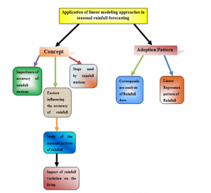
Figure 2.1: Conceptual Framework
(Source: Created by Researcher)
2.3.1 Importance of accuracy of rainfall stations
Rainfall, a major meteorological phenomenon has the greatest impact on human activities and associated anthropogenic tasks related to the same. For the sake of avoiding the damage brought about by excessive rainfall or catching the opportunities of rainfall bolstered agricultural growth, accurate forecasting of seasonal rainfall in extremely important. Hence, gauging the intensities of rainfall in the correct manner is the prima facie necessity of meteorological departments and this should be done keeping an eye on both beneficial and detrimental effects of rainfall on human life and processes of human society in bona fide terms or manners. As per Monteiro et al. (2016, p.1426),both cross-sectional and time series study of different intensities of rainfall in an accurate manner is vital for study in the major rain affected territories of the world in a by and large manner.
Accuracy is extremely essential for the sake of the fact that appropriate rainfall data will help to predict requisite growth in the agricultural sector or environmental damages connected by its harshness with efficiency. The relationship between the intensity of rainfall and various types of agricultural and associated primary activities are most crucial factors of study, keeping into consideration the benefits of rainfall on cropping pattern which is directly related with development. The railway stations are considered as most relied stations for predicting rainfall amounts in different seasons which is vital for a variety of economic processes and the accuracy level in lieu of their measurement is extremely significant.
As per Keller et al. (2015, p. 143),the significance of accurate detection of rainfall intensities for opening the opportunities for rainfall pre-predicted development has made the establishment of rainfall stations vital for most of the rain prone regions of the globe. Both quantity and quality of rainfall can be measured in terms of meteorological forecasts done by the use of rainfall stations in regions vulnerable to consistent rainfall in all periods of the year in accurate manners.
2.3.2 Steps used by rainfall stations
Computation of rainfall can be done by use of various methods of methods of measurement of seasonal rainfall as standardised by WMO(World Meteorological Organisation).The three common methods and the steps of measurement are underlined below:
- Arithmetic average method-In this method first of all the rainfall led rain depths at different locations surrounding the particular rainfall station or in different railway is gauged and measured. Based on the strength of uniformity of data in terms of rain depths, the gross sum of total additive sums of various rain depths is obtained and then they are divided by the number of railway stations to arrive at figures detecting the amount of rainfall. These methodological steps are used to detect intensities of storm rainfall in monthly or yearly average respectively.
b.Weighing mean method or Thiessen Polygon method-This method of rainfall measurement is based on gauging rainfall intensities in moderate amounts taking into consideration very few rain affected regions around railway stations.The first step is based on drawing a scale of measurement of rainfall data in terms of sketching of boundaries and locations of rain gauges in corresponding areas under consideration. Then joining of the rain gauges to form the network of triangles is done. Then drawing of the perpendicular bisectors of triangles is done.After that delineation of formed polygons and measurement of their areas by a plani-meter is performed by taking smaller geometric shapes (Olawoyin and Acheampong, 2017, p.158). Then finally average of precipitation data is calculated.
.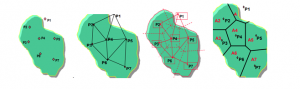
Figure 2.2: Steps of measurement of rainfall in Thiessen Polygon Method
(Source:Olawoyin and Acheampong, 2017, p.158)
c.Isohyetal method-The isohyetal method of measurement of rainfall considers the measurement of rainfall in rugged and rough areas of rain affected zones around rainfall stations. The first step is to draw the area of study and by scaling it in terms of location of rain gauges in it. The second step is to draw isohyets of different values by putting into consideration the rainfall data. The third step is the determination of area under each pair of isohyet lines (Fikre et al. 2016, p. 8). The fourth and step are to calculate average rainfall with the help of these areas under isohyets lines respectively.
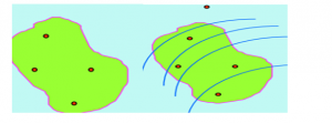
Figure 2.3: Steps for measurement of rainfall in an Isohyetal method
(Source:Fikre et al. 2016, p.8).
2.3.3 Factors influencing the accuracy of rainfall measurements
As per Trenberth et al. (2014, p.17), the prime factors influencing the accuracy of rainfall measurements can be both anthropogenic factors and man-made and non-anthropogenic factors are as follows:
Natural or non-man made factors
a.Solar intensity linked factor-Variation in solar intensities act as barriers in the way of the correct measure of precipitation by rainfall stations.This is because of the presence of harmful and strong wavelength based ultraviolet and infrared radiations act as barriers in the way of successful measurements of intensities of rainfall both in average and absolute terms. These sun rays prove detrimental effects on the surface of rain gauge and hamper its effectiveness to be used as a good rainfall measuring tool.
b.Orbital shift linked factor- The movement of earth’s rotation around the sun cause irregularities in the amounts of energy reaching the earth and this causes variation in the measurements of rainfall as accurate data of rainfall occurring in an area is hurt. This is due to the presence of solar intensity based irregularities in earth’s surface and disruptions in gauging of rainfall intensities in the correct manner (Diederich et al. 2015, p.508).
- Volcanic activity linked factor-Level of volcanic activities also cause irregularities in patterns of rainfall due to disruptions of sun’s rays reaching the earth and hence this cause aberration in the way of successful measurement of rainfall.
d.Continental drift based factor-The occurrence of continental drifts cause changes in climatic and weather conditions and this causes variations in atmospheric conditions leading to an inaccurate or imprecise level of detection of exact rainfall intensities by rainfall stations even after using superior tools of rainfall measurement.
Man-made factors
a.Greenhouse gas emission based factor-The presence of greenhouse gases also disrupts measurement accuracy of rainfall data by rainfall stations in specific amounts. The disequilibrium created in energy balance affects the rainfall measurement adversely.
b.Fossil fuel overuse based factor-Extreme use of fossil fuels also causes aberrations in the path of suitable measurement of measurement of rainfall data by rainfall stations.
2.3.4. Study of the seasonal pattern of rainfall
As per Fischer and Knutti(2015, p.560), global patterns in precipitation in terms of seasonal variation in intensities over the year is affected by the movement of winds and their deflection in rain-prone areas of the world. The winds such as trade winds, westerlies and cyclones cause changes in the seasonal variation and irregularities immune-precipitation amounts and quality across the globe in handsome and specific amounts as per time periods. The prevalence of temperature modifications due to side effects of global warming and greenhouse emission cause irregularities
in the speed of precipitation amounts in different seasons of the year in various high and low-pressure belts of countries troubled by consistent precipitation across the globe respectively.

Figure 2.4: Global patterns in precipitation
(Source:Fischer andKnutti, 2015, p.560)
As precipitation variation is seen to affect various climatic factors and criterion of climate such as thermo-haline circulation, chemical mass balance and productivities of ocean water surfaces in and around the globe, hence study of seasonal variations in rainfall is extremely important. According to Zhang and Zhou (2014, p.168), the major climatic phenomenon and the weather-related phenomenon of change in temperatures and change in water level of oceans seas and large river systems caused by seasonal variation in rainfall.This is linked with economic and non-economic activities in the world. The arising of tides and floods and droughts created in different seasons of the year due to seasonal variance rainfall intensities has huge implications for transportation and marketing based business world phenomenon. The cultural and socioeconomic life of people is widely modified by changes in environmental conditions brought about by changes in seasonal patterns in rainfall through various natural processes respectively.
Use of modern methods for studying the intensity of precipitation in various parts of the world in different seasons is the major interest of research study by meteorological and climatic experts in different parts of the world. The use of infrared radiations and microwave rays are stupendously popular ways of current era to do the same as per certain measurement criterion of precipitations in and across the world. Use of longitudinal-latitudinal data in different parts of the world is the very common ingredient or aspect of measurement of seasonal diversity in precipitation in and across the world.
2.3.5 Relation of Rainfall with other climatic changes
Precipitation intensities are inherently linked with different varieties of climatic changes occurring and across the globe. As per Romps et al. (2014, p.854), the significance of precipitation in affecting the global warming patterns has a direct linkage in terms of its impact on modifications in temperatures of regions hit by frequent precipitation in different amounts in different seasons of the year.
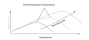
Figure 2.5: Precipitation and global warming
(Source: Fischer and Knutti, 2015, p.560).
Since warmer air is more moisture retentive than dryer air hence global warming has a direct relevance to the increase in precipitation intensities. Hence dangers of global warming are up on the rise with the increase in precipitation levels of various tropical and temperate regions of the world witnessing high levels of precipitation over the years. The equatorial region surrounding the Amazonian territories of the world are the major areas of the world witnessing major quantity of precipitation around the world. Changes in weather behaviour and deflection of winds brought about by cyclonic storms and tempests lead to massive climatic adversities in and around the world.
Droughts and floods brought about by extremely heavy levels and scanty levels of precipitation respectively show the direct linkage between rainfall and other climate-related processes occurring in different parts of the world. According toOslandet al.(2016, p.8). Too much precipitation is connected with warmer climate whereas colour climate is witnessed in vice versa scenario of precipitation. The modifications of land and sea breezes and other climate-related continental phenomenon both in oceans and land surfaces are related to precipitation intensity in a wide manner.
2.3.6 Impact of rainfall variation on the living environment
Consistently high rainfall is the purveyors of many varieties of chronic diseases of both endemic and epidemic varieties in extremely rain sensitive areas of the globe. Torrential precipitation is seen to be the harbinger of growth many kinds of disease-causing bacteria and amoeba and various classes of protozoa which affect sick, old and children quickly with various malignant diseases. If not stopped or taken precautions to get rid of these rainfall disease-causing microbes, then they are seen to take lives of humans without any limitations.
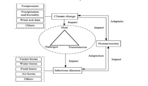
Figure 2.6: Impact of rainfall based climatic change on living environment
(Source:Tomczyket al. 2016, p.166)
According to Tomczyket al. (2016, p. 166), similarly, the nitric oxides created in the process of precipitation in the atmosphere often proves fatal for the fertility of earth surface once they touch the earth and destroys the natural ingredients of fertile soil.Thus destruction in intensity of crop generation affects the agricultural activities adversely leading loss of money and lives of poor people thriving on agricultural activities on earth. This hurt the economic processes connected with human life in an intensive manner and lead to both environmental and economical losses of human inhabitants on earth in bona fide terms. Occurrence of floods due to excessive rainfall affects the man-made transportation systems adversely for which the business lives of professional and non-professional people are hurt. Cyclonic storms and tempests related with giant rainfall both in intensity and duration affect the anthropogenic and man-made settlements and institutions adversely bringing devastation of properties and loss of human life directly by death or indirectly by scarcity due to economic loss.
2.4.1 Correspondence analysis of Rainfall data
Since the middle of the 90s, a number of studies and researches were developed for seasonal rainfall forecast, in order to help the business and landowners to adapt to any type of decisions. Unfortunately, it can be said that after two decades, the forecasting skills and approaches are still situated at a lower level and this cannot be efficiently applied in the decision making process. Therefore, as stated by Bagirovet al. (2017, p.25), a larger portion of the population is still suffering due to the high level of discrepancies among rainfall forecasting estimation processes.
Application of statistical approaches for analysing the rainfall data is essential for many aspects such as various engineering constructions, estimation of relevant input output value for construction and also for crop planning. A daily rainfall data period is necessary to identify and evaluate the value of normal rainfall, seasonal rainfall, excess rainfall and deficit rainfall. Bordoniet al. (2015, p.30) stated that the analysis of rainfall data by statistical methods leads to the development of much accurate output which is applicable as a resource for different work field people. Different statistical methods, such as regression analysis, mean and standard deviation, coefficient of variation of monthly and yearly rainfall data is generally used for checking the variability of rainfall. According to the statement of Broccaet al. (2014, p.5140), through the calculated result, the determination of rainfall pattern becomes easier.
2.4.2 Importance of statistical approaches in measuring Rainfall data
Evaluation of rainfall forecasting can be conducted by the applications of the above mentioned statistical analysis methods. Chen et al. (2014, p.335) opined that the statistical data can be considered as reliable and accurate as they develop from a number of steps like collection, analysis, validation and so on. In addition, it can also be stated that statistical data is not only applicable in the field of mathematics, it can also be applied in different field of researches in order to organise, summarise and analyse the collected information. As stated by Deo et al. (2017, p.170), the data and information used in the statistical analysis patterns are often used to support the pre-existing hypotheses and it also provides credibility in research methodology and data analysis parts.
Through statistical data analysis process, researchers can understand and describe the patterns of rainfall in different parts of the world and can interpret an appropriate result from it. Various types of linear methods are applied for the selection of the predictors and the development of seasonal rainfall forecasting models. Some of the mostly applicable analysis methods are correlation analysis, stepwise regression, cross validation, principal component analysis or PCA and linear regression.
2.4.3 Linear Regression pattern of Rainfall data
In order to evaluate rainfall forecast, one of the most commonly used predictive analysis method is linear regression pattern. This concept is generally based on two variables, set of predictor variables and effects of the outcome variables. Haddad et al. (2015, p.75) stated that the patterns of regression analysis is useful for analysing the relationships among the above two mentioned variables. In case of linear regression analysis method the most simplest form of regression equation is y=c+b*x, where y stands for value of estimated dependent variable, c is constant, b represents the regression coefficient and value of the independent variable. According to the statement of Innes et al. (2015, p.100), the most common uses of regression analysis are determination of the strengths of predictors, trend forecasting and forecasting of impacts.
Regression analysis can predict the trends and future scores of environmental as well as technological situations. Isottaet al. (2014, p.1670) mentioned that linear regression analysis can be used for getting the estimation point. Seasonal rainfall forecasting can be understood by several types of linear regression patterns such as simple linear, multiple linear, logistic, multinomial, ordinal and discriminate analysis method. Due to the simplicity of pattern, simple linear regression analysis is mostly used for rainfall forecasting. Lim et al. (2016, p. 2289) stated that simple linear regression is dependent on one dependent variable and one independent variable. Through this, the impact of one variable (independent variable) over the other (dependent variable) can be estimated. It can be said that the simple and multiple linear method is different from each other in the aspects of variable numbers. On the contrary, Pfahlet al. (2017, p.423) stated that simple linear method is overly simplistic, that cannot be applied in many of the real life circumstances.
2.4.4 Application in Rainfall Forecasting
Establishment of a linear pattern of relationship among the predictor and explanatory variables comes along with the inherent predictive scores. In different aspects of life, either natural or artificial, forecast is crucial as it can help in determining the number of possible occurrences. Different strategies can be prepared based on these forecasting values by altering or managing the resources. Thus, as mentioned by Poulteret al. (2014, p.600), different linear regression models are developed to enhance the efficiency level of rainfall forecasting.
(Source: Science.psu.edu, 2018)
As mentioned earlier, the simple linear regression analysis is dependent on two factors which are designated as X and Y. Through mathematical convention, the simple equation which can describe the relationship between X and Y, is termed as the regression model. Besides this, Poulteret al. (2014, p.600) identified that the linear regression model also includes a term named Error, designated by E or epsilon. This error is a vital factor, which is used for accounting the variability in Y, that cannot be described or explained by the linear regression equation of X and Y. The equation for simple linear regression used for estimating seasonal rainfall approach is Ε(y) = (β0 +β1 x). Rahman et al. (2018, p.130) mentioned that in order to conduct assumption and estimation, simple linear regression model is suitable. Moreover, this model can also be applied for parameter estimation and inference prediction.
Chapter 3: Research Methodology
Research methodology refers to a systematic way for solving the research issues by the logical adaptation of various myriad steps. The aim of research methodology is to provide a brief and clear descriptions of the research methods, shed light on the gaps and limitations, and clarify their consequences. In this chapter, an appropriate research methodology has been carried out to allow the researchers for effective and successful completion of the dissertation. In order to complete the dissertation, researchers has collected information from different theoretical substructures and existing conceptual models in the previous chapter. Suitable research philosophy, research approach, research design, sampling techniques and justifications for choosing them are described by researchers. At last, the ethics and an overall summary of the research methodology have also been evaluated here.
| Types | Methods Used |
| Research Philosophy | Positivism |
| Research Approach | Deductive |
| Research Design | Explanatory |
| Data collection method | Secondary |
| Data collection tool | Quantitative |
| Sampling techniques | Simple random probability |
| Sampling size | 50 rainfalls from NSW |
| Data analysis tool | SPSS |
Table 3.1: Research Outline
(Source: Created by researchers)
In order to conduct a research successfully, researchers need to adopt a proper research philosophy, which is required to carry out the objectives of this research. Realism research philosophy helps in the determination that the results or outcomes of the researchers will not be biased after research. Brannen(2017, p.12) mentioned that in this philosophy, social reality is generally accepted to fulfil a research aims. On the contrary, interpretivism philosophy represents the individual human perception for judging any matters related to the research. Eriksson and Kovalainen(2015, p.34) stated that through the application of positivism research philosophy, researcher can take help of the pre-existing theories and models to generate a hypothesis, which would be analysed in the entire research method. Therefore, it can be stated that in order to complete this particular research, positivism research philosophy has been applied.
3.4.1 Justification for choosing positivism philosophy
To carry out the specific objectives of the research, positivism research philosophy is suitable for collecting a range of information about monthly or yearly rainfall forecasting in Australia. The importance and accuracy level of the statistical analysis methods for obtaining future relationships among variables have been used for the development of this research. As stated by Gastand Ledford (2014, p.55), existing theories and concepts of simple linear regression models have been taken into consideration for conducting the estimation of seasonal rainfall forecasting. In addition, the concepts and models have also helps in the formulation of the research aims and objectives. Since this research needs statistical analysis, therefore, Kelly et al. (2014, p.61) mentioned that positivism philosophy is appropriate as it generally relies on the quantifiable information or observation. Through the application of positivism philosophy, the collected information and data has only been evaluated only by logical and scientific way.
Most commonly used research approaches are deductive and inductive. Among them, for conducting this particular research, deductive approach is suitable as it mainly focuses on the retaining knowledge. Mackey andGass(2015, p.35) opined that this research approach uses the top to bottom approach, which provide the opportunity to the researchers for formulating the research aims through proper review of the existing literatures. This can be proved through the conduction of the entire research and analysis of the gathered data of seasonal rain falling. On the contrary, Merriam and Tisdell(2015, p.67) stated that if creation of new theories and hypotheses are required, in those cases inductive theories can be applied. Therefore it can be said that the main difference among the deductive and inductive approach is whilst inductive approach is associated with the creation or generation of novice theories, a deductive approach is aimed to test the pre-existing theories and concepts.
3.5.1 Justification for choosing deductive approach
Based on the differences among the two research approaches, the researcher has decided for the deductive research approach to conduct this particular research. Mertens(2014, p.29) mentioned that deductive approach helps in the exploration of the suitability of a known or existing theories or concepts in a specific circumstances. In addition to this, deductive approach can explain the causal relationship among the given variables and existing concepts of rainfall forecasting. It is more likely applicable in the case of quantitative researches, but there may be exception. As opined by Meyers et al. (2016, p.10), deductive approach starts with old concepts and ends with the development of research objectives. The researchers can use the old concepts and models for proving the authenticity of the research topic.
Three types of research design can be applied to conduct a research successfully, which are descriptive, explanatory and exploratory. In order to complete a research, the research design is generally selected based on the research aims and objectives. Smith (2015, p.18) stated that exploratory method includes the psychological variables whereas the descriptive method can be applied in the analysis of specific objectives and questions. Thus, in this case, since a set of questions are not present, the explanatory method has considered as the most suitable design for this dissertation. Silverman (2016, p.40) opined that the explanatory research design allows the researchers to understand the evidences and concepts more efficiently. In addition to the explanatory research can also help in connecting different ideas and understanding different causes and their impacts as it is more flexible than the other two types of designs.
3.6.1. Justification for choosing explanatory design
To conduct this specific research efficiently, researchers has adopted explanatory design as this research does not have any set of questionnaires. In this research, any types of description of the pre-existing models or concepts have not required. The explanatory design is appropriate for this particular dissertation since according to the statement of Strangand Braithwaite (2017, p.79), researchers have collected and analysed the data and information about seasonal rain falling. In addition to that, explanatory design is mostly dependent on the flexibility of resources, which includes a number of published literature, articles and e-books. It helps in conducting an in depth analysis of the research subject.
Data can be classified as primary and secondary, which can further be divided as quantitative and qualitative. Through the conduction of different field works like survey and interview the primary data can be gathered, whereas the secondary data or information is collected through the examination and evaluation of existing literatures. Taylor et al. (2015, p.54) stated that qualitative data generally includes a sort of justification of a problem relevant to the research topic in a descriptive manner. On the contrary, quantitative data is used for generating statistical representation of the collected numerical data in the forms of chart, tables and graphs. Brannen(2017, p.88) started that both primary and secondary research method can use the qualitative and quantitative data collected by the researchers. However, in this case, for analysing the seasonal rainfall forecasting, secondary quantitative data and information have been used.
3.7.1. Justification for choosing secondary quantitative data
In this research, primary data cannot be obtained as rainfall is a natural phenomenon, therefore, any primary data related to this topic does not exist. Thus in this case, researchers have applied secondary quantitative data collection method. Mertens(2014, p.30) stated that secondary data can be obtained from many authentic resources, such as published literatures, organisational surveys, government reports or authentic online databases. For conducting this research, numerical information of 50 rainfall stations from NSW report has been collected, which have been represented by the form of charts, graphs and tables. In addition, Silverman (2016, p.22) mentioned that secondary quantitative research method provides the opportunity to the researchers to collect data in a very short time as well as cost effective manner. Moreover, this research method can make the future primary data collection method much specific by identifying the gaps and deficiencies from the collected information.
3.8 Sampling Techniques and Size
Sampling refers to a process of unit selection from a population of choice from where the researchers can generate an authentic and almost accurate result or outcome. Saunders et al. (2009, p.43) opined that sampling techniques is completely dependent on some terms such a sampling frame and population. For completing research, most of the researchers use the random probability sampling techniques as it provides assurance that each and every unit of the targeted population may get equal opportunities of being selected. Tsangaratos and Ilia (2016, p.170) analysed that different random sampling techniques can be used in analysing the collected information such as simple, stratified, multistage, cluster and systematic sampling technique. Among them, most useful techniques is simple random probability sampling method as it is the simplest techniques by which researchers can generate appropriate results.
3.8.1 Justification for choosing random probability sampling
To analyse the information about seasonal rainfall forecasting, the samples have been chosen from the government reports of NSW among the huge number of rainfall reports, 50 rainfall stations have been chosen randomly by the researchers. Schulze et al. (2014, p.1130) mentioned that for developing authentic results, it is necessary to evaluate all types of rainfall records from the available data and therefore random technique is followed for this research.
For analysing the numerical analysis using linear regression models, the most commonly used data analysis tool is SPSS or Statistical Packages for Social Sciences. Sadyśet al. (2015, p.27) stated that it is one the comprehensive and logical system for analysing the collected numerical data. SPSS can use information from any types of sources and generate a number of charts, tabular reports and plots through regression analysis, t-square test, chi square tests, binomial selection and so on.
3.9.1. Justification for choosing SPSS
Since this research is based on quantitative data collection method, thus researchers have used SPSS software to analyse the collected quantitative data. In the modern IBM SPSS software package, total 15 numbers of modules are present for analyse the collected data based on the research process requirement. Strangand Braithwaite (2015, p.70) stated that, SPSS modules are user friendly and generates accurate results, therefore researchers can predict future forecasts in a quick and easy way. This software is mainly designed for all research scholars to conduct the analysis part of the research and attaining their desired outcomes with an appropriate graphical representation.
It is often thought that secondary research method can provide relief to the researchers such as this research method does not need any ethical approval. However, a number of ethical considerations is enlisted for this particular research also. Yang and Yu (2015, p.180) stated that this types of secondary quantitative researches are needed to conduct for the public well being. Moreover, the results or outputs are needed to ensure transparency and reliability. Researchers has collected the data from authentic resources and followed de-identification of the collected information before applying in the research. In addition, the data of seasonal rainfall has collected only from government websites. Through the application of SPSS, researchers have acquired authentic and accurate outputs of the seasonal rainfall forecasting.
[Refer to Appendix]
The above methodology chapter describes the entire process of research method including the philosophy, approach and designs. All of the variables have been selected according to the research criteria and requirement. To conduct the research, positivism research philosophy and deductive approach has been followed by the researchers. Through the use of explanatory research design, researchers have been developed an appropriate outcome through the analysis of the information. Since primary data collection is not possible in this research, authentic source of secondary quantitative data has been analysed. In order to acquire authentic information about seasonal rainfall, 50 rainfall stations have been chosen by simple random probability sampling technique from a NSW government report. With the chosen data, SPSS analysis has been done through simple linear regression analysis.
Chapter 4: Results and Discussion
4.1.1. Regression analysis of rainfall of 3 hours in NSW’s rainfall stations on total yearly rainfall
N (number of observations) =50
Regression equation: Y=a+bX +U
Y= Total yearly rainfall (endogenous variable), X=3 hrs rainfall, U=random term
a=intercept, b=regression coefficient
| N(Number of observations) | Y(total yearly rainfall) | X(3 hrs rainfall) |
| 1 Cudgera | 1577.0 | 164.5 |
| 2 Main Arm | 2116.0 | 156.0 |
| 3 Huonbrook | 2182.0 | 123.0 |
| 4 Myocum | 1799.0 | 100.0 |
| 5 Lake Ainsworth | 1825.5 | 73.0 |
| 6 Wooli Caravan | 1825.5 | 40.5 |
| 7 Perry Drive | 1715.0 | 42.0 |
| 8 Shepards Lane | 1726.0 | 50.0 |
| 9 Red Hill | 1845.0 | 53.5 |
| 10 Newports Creek | 1934.5 | 59.0 |
| 11 Middle Boambee | 1982.5 | 40.0 |
| 12 North Bonville | 1977.5 | 52.0 |
| 13 Koorowi | 1793.5 | 40.5 |
| 14 Stuart Island Downstream | 1270.5 | 49.5 |
| 15 Utungun | 1410.0 | 43.0 |
| 16 Green Valley | 1224.0 | 33.0 |
| 17 Aldavilla Downstream | 1079.0 | 37.5 |
| 18 Telegraph Point | 1243.5 | 45.0 |
| 19 Logans Crossing | 807.0 | 53.5 |
| 20 Mount George | 1247.5 | 40.0 |
| 21Nabiac | 935.5 | 31.5 |
| 22Tuncurry Downstream | 1103.5 | 35.5 |
| 23Pacific Palms Wharf | 1142.5 | 44.0 |
| 24 Tarbuck Bay | 1265.5 | 34.5 |
| 25Bulahdelah | 1053.0 | 34.0 |
| 26Gostwyck | 853.0 | 33.5 |
| 27 Seaham | 988.0 | 58.0 |
| 28 Belmore Bridge | 896.5 | 25.0 |
| 29Hexham Bridge | 819.5 | 29.0 |
| 30Barnsley | 898.5 | 37.5 |
| 31 Martinsville | 1028.5 | 27.0 |
| 32 Mandalong | 1019.5 | 40.0 |
| 33 Wyee | 1156.5 | 30.5 |
| 34 Whitemans Ridge | 1104.5 | 31.0 |
| 35Yarramalong | 821.0 | 64.5 |
| 36Kulnura | 2301.5 | 40.0 |
| 37 Toukley | 909.5 | 47.5 |
| 38Hamlyn Terrace | 1246.5 | 49.5 |
| 39Mardi Dam | 1223.5 | 31.5 |
| 40Sterland | 1324.5 | 44.5 |
| 41Kangy Angy | 1260.0 | 53.5 |
| 42Berkeley Vale | 1200.3 | 36.0 |
| 43Bateau Bay | 1149.5 | 40.0 |
| 44Lisarow | 1473.0 | 46.0 |
| 45Strickland | 1475.5 | 50.0 |
| 46Narara | 1373.5 | 35.5 |
| 47Mount Elliot | 2602.0 | 72.5 |
| 48Wyoming | 852.8 | 30.8 |
| 49Kincumber | 795.2 | 26.6 |
| 50Webbs Creek | 573.2 | 27.6 |
Table 4.1: Tabular representation of 3hrs of rainfall and total yearly rainfall in 50 NSW rainfall stations of Australia
| Descriptive Statistics | |||
| Mean | Std. Deviation | N | |
| Y(total yearly rainfall) | 1348.58 | 457.114 | 50 |
| X(3 hrs rainfall) | 49.72 | 28.822 | 50 |
| Model Summary | |||||||||
| Model | R | R Square | Adjusted R Square | Std. The error of the Estimate | Change Statistics | ||||
| R Square Change | F Change | df1 | df2 | Sig. F Change | |||||
| 1 | .499a | .249 | .233 | 400.220 | .249 | 15.921 | 1 | 48 | .000 |
| a. Predictors: (Constant), X(3 hrs rainfall) | |||||||||
| Coefficients | ||||||||
| Model | Un-standardised Coefficients | Standardized Coefficients | t | Sig. | 95.0% Confidence Interval for B | |||
| B | Std. Error | Beta | Lower Bound | Upper Bound | ||||
| 1 | (Constant) | 955.027 | 113.717 | 8.398 | .000 | 726.385 | 1183.670 | |
| X(3 hrs rainfall) | 7.915 | 1.984 | .499 | 3.990 | .000 | 3.927 | 11.904 | |
| a. Dependent Variable: Y(total yearly rainfall) | ||||||||
Discussion: The regression done above illustrates the significance of the relationship between 3 hrs rainfall figures in 50 chosen rainfall stations of NSW in Australian economy(exogenous variable) and total yearly rainfall in those states in Australia (endogenous variable) respectively. The goodness of fit value namely R depicts the intensely good fit of regression data which is 0.249 at positively high significance level. The adjusted R square value is about 0.233 which is also found to be significant at the high level of significance.
The value of regression coefficient (b) is 7.915 which indicate strong positive regression relationship between the 3 hrs rainfall of 50 rainfall stations and total yearly rainfall of them respectively.The standardised beta is 0.499 with the standard error value of 1.984 respectively. The calculated t statistic is found to be significant at the value of 3.99 at 95% confidence interval. Thus, the p-value is lower than the level of significance value of 0.05. It indicates rejection of the null hypothesis of no relationship between 3 hours of the rainfall of 50 stations and total yearly rainfall of the same respectively. Thus, the linear regression model is efficient in bringing out the positivity of estimating the seasonal variation in rainfall in 50 stations via regression relationship between the two considered variables.
4.1.2. Regression analysis of rainfall of 6 hours in NSW’s rainfall stations on total yearly rainfall
N (Number of observations) =50
Regression equation: Y=a+bX+U
Y=Total yearly rainfall (endogenous variable), X= 6 hours rainfall (exogenous variable)
U=random term
a=intercept, b=regression coefficient.
| N(Number of observations) | Y(total yearly rainfall) | X(6 hrs rainfall) |
| 1 Cudgera | 1577.0 | 248.0 |
| 2 Main Arm | 2116.0 | 233.5 |
| 3 Huonbrook | 2182.0 | 172.5 |
| 4 Myocum | 1799.0 | 144.5 |
| 5 Lake Ainsworth | 1825.5 | 114.5 |
| 6 Wooli Caravan | 1825.5 | 54.5 |
| 7 Perry Drive | 1715.0 | 73.5 |
| 8 Shepards Lane | 1726.0 | 85.0 |
| 9 Red Hill | 1845.0 | 94.0 |
| 10 Newports Creek | 1934.5 | 94.5 |
| 11 Middle Boambee | 1982.5 | 73.0 |
| 12 North Bonville | 1977.5 | 79.0 |
| 13 Koorowi | 1793.5 | 63.5 |
| 14 Stuart Island Downstream | 1270.5 | 69.5 |
| 15 Utungun | 1410.0 | 74.5 |
| 16 Green Valley | 1224.0 | 60.0 |
| 17 Aldavilla Downstream | 1079.0 | 59.0 |
| 18 Telegraph Point | 1243.5 | 75.5 |
| 19 Logans Crossing | 807.0 | 77.5 |
| 20 Mount George | 1247.5 | 45.5 |
| 21Nabiac | 935.5 | 38.5 |
| 22Tuncurry Downstream | 1103.5 | 45.0 |
| 23Pacific Palms Wharf | 1142.5 | 47.0 |
| 24 Tarbuck Bay | 1265.5 | 42.0 |
| 25Bulahdelah | 1053.0 | 34.5 |
| 26Gostwyck | 853.0 | 36.5 |
| 27 Seaham | 988.0 | 60.5 |
| 28 Belmore Bridge | 896.5 | 32.5 |
| 29Hexham Bridge | 819.5 | 33.0 |
| 30Barnsley | 898.5 | 40.0 |
| 31 Martinsville | 1028.5 | 44.0 |
| 32 Mandalong | 1019.5 | 43.5 |
| 33 Wyee | 1156.5 | 39.0 |
| 34 Whitemans Ridge | 1104.5 | 37.0 |
| 35Yarramalong | 821.0 | 82.5 |
| 36Kulnura | 2301.5 | 47.5 |
| 37 Toukley | 909.5 | 47.5 |
| 38Hamlyn Terrace | 1246.5 | 52.5 |
| 39Mardi Dam | 1223.5 | 61.0 |
| 40Sterland | 1324.5 | 47.0 |
| 41Kangy Angy | 1260.0 | 56.5 |
| 42Berkeley Vale | 1200.3 | 65.0 |
| 43Bateau Bay | 1149.5 | 42.5 |
| 44Lisarow | 1473.0 | 46.5 |
| 45Strickland | 1475.5 | 46.5 |
| 46Narara | 1373.5 | 75.5 |
| 47Mount Elliot | 2602.0 | 45.5 |
| 48Wyoming | 852.8 | 37.6 |
| 49Kincumber | 795.2 | 30.2 |
| 50Webbs Creek | 573.2 | 29.6 |
Table 4.2: Tabular representation of 6hrs of rainfall and total yearly rainfall in 50 NSW rainfall stations of Australia
|
Descriptive Statistics |
|||
| Mean | Std. Deviation | N | |
| Y(total yearly rainfall) | 1348.58 | 457.114 | 50 |
| X(6 hrs rainfall) | 67.52 | 45.276 | 50 |
| Model Summary | |||||||||
| Model | R | R Square | Adjusted R Square | Std. Error of the
Estimate |
Change Statistics | ||||
| R Square Change | F Change | df1 | df2 | Sig. F Change | |||||
| 1 | .496a | .246 | .231 | 400.969 | .246 | 15.683 | 1 | 48 | .000 |
| a. Predictors: (Constant), X(6 hrs rainfall) | |||||||||
| Coefficients | ||||||||
| Model | Unstandardized Coefficients | Standardized Coefficients | T | Sig. | 95.0% Confidence Interval for B | |||
| B | Std. Error | Beta | Lower Bound | Upper Bound | ||||
| 1 | (Constant) | 1010.285 | 102.532 | 9.853 | .000 | 804.131 | 1216.439 | |
| X(6 hrs rainfall) | 5.010 | 1.265 | .496 | 3.960 | .000 | 2.467 | 7.554 | |
| a. Dependent Variable: Y(total yearly rainfall) | ||||||||
Discussion: The regression tables based results depicted above shows the significance of regression relationship between 6 hours of the rainfall of 50 rainfall stations and the total yearly rainfall of the stations. The R square based goodness of fit relationship is found to be of value =0.246.The adjusted R square to be of value =0.231 which explains the fit of sound regression data in the linear regression model with highly significant levels. The regression coefficient (b) is found to be of positive value 5.010 and its standardised form =0.496.The t-statistic (calculated) is found to be =3.960 which is found to highly significant at 95% C.I with p-value lesser than the level of significance. Thus, with the rejection of the null hypothesis, the significance of the positive impact of 6 hours rainfall on total yearly rainfall is derived by linear regression method.
4.1.3. Regression analysis of rainfall of 12 hours in NSW’s rainfall stations on total yearly rainfall
N (Number of observations)=50
Regression equation: Y=a+bX
Y=total yearly rainfall (endogenous variable), X= 12 hours rainfall(exogenousvariable)
U=random term
a=intercept, b=regression coefficient)
| N(Number of observations) | Y(total yearly rainfall) | X(12 hrs rainfall) |
| 1 Cudgera | 1577.0 | 288.5 |
| 2 Main Arm | 2116.0 | 282.0 |
| 3 Huonbrook | 2182.0 | 264.5 |
| 4 Myocum | 1799.0 | 173.5 |
| 5 Lake Ainsworth | 1825.5 | 135.5 |
| 6 Wooli Caravan | 1825.5 | 83.5 |
| 7 Perry Drive | 1715.0 | 118.6 |
| 8 Shepards Lane | 1726.0 | 135.5 |
| 9 Red Hill | 1845.0 | 151.6 |
| 10 Newports Creek | 1934.5 | 157.6 |
| 11 Middle Boambee | 1982.5 | 132.0 |
| 12 North Bonville | 1977.5 | 132.0 |
| 13 Koorowi | 1793.5 | 89.0 |
| 14 Stuart Island Downstream | 1270.5 | 118.0 |
| 15 Utungun | 1410.0 | 110.5 |
| 16 Green Valley | 1224.0 | 95.0 |
| 17 Aldavilla Downstream | 1079.0 | 97.6 |
| 18 Telegraph Point | 1243.5 | 113.5 |
| 19 Logans Crossing | 807.0 | 114.5 |
| 20 Mount George | 1247.5 | 54.0 |
| 21Nabiac | 935.5 | 65.5 |
| 22Tuncurry Downstream | 1103.5 | 50.5 |
| 23Pacific Palms Wharf | 1142.5 | 57.5 |
| 24 Tarbuck Bay | 1265.5 | 47.0 |
| 25Bulahdelah | 1053.0 | 34.6 |
| 26Gostwyck | 853.0 | 46.0 |
| 27 Seaham | 988.0 | 62.0 |
| 28 Belmore Bridge | 896.5 | 37.0 |
| 29Hexham Bridge | 819.5 | 43.6 |
| 30Barnsley | 898.5 | 50.5 |
| 31 Martinsville | 1028.5 | 56.5 |
| 32 Mandalong | 1019.5 | 46.5 |
| 33 Wyee | 1156.5 | 57.5 |
| 34 Whitemans Ridge | 1104.5 | 47.0 |
| 35Yarramalong | 821.0 | 119.5 |
| 36Kulnura | 2301.5 | 49.6 |
| 37 Toukley | 909.5 | 79.0 |
| 38Hamlyn Terrace | 1246.5 | 95.5 |
| 39Mardi Dam | 1223.5 | 60.5 |
| 40Sterland | 1324.5 | 86.5 |
| 41Kangy Angy | 1260.0 | 102.0 |
| 42Berkeley Vale | 1200.3 | 66.0 |
| 43Bateau Bay | 1149.5 | 60.5 |
| 44Lisarow | 1473.0 | 59.0 |
| 45Strickland | 1475.5 | 107.5 |
| 46Narara | 1373.5 | 64.6 |
| 47Mount Elliot | 2602.0 | 129.0 |
| 48Wyoming | 852.8 | 44.8 |
| 49Kincumber | 795.2 | 42.0 |
| 50Webbs Creek | 573.2 | 30.6 |
Table 4.3: Tabular representation of 3hrs of rainfall and total yearly rainfall in 50 NSW rainfall stations of Australia
|
Descriptive Statistics |
|||
| Mean | Std. Deviation | N | |
| Y(total yearly rainfall) | 1348.58 | 457.114 | 50 |
| X(12 hrs rainfall) | 94.98 | 59.368 | 50 |
| Model Summary | |||||||||
| Model | R | R Square | Adjusted R Square | Std. The error of the Estimate | Change Statistics | ||||
| R Square Change | F Change | df1 | df2 | Sig. F Change | |||||
| 1 | .617a | .381 | .368 | 363.512 | .381 | 29.483 | 1 | 48 | .000 |
| a. Predictors: (Constant), X(12 hrs rainfall) | |||||||||
| Coefficients | ||||||||
| Model | Un-standardised Coefficients | Standardized Coefficients | t | Sig. | 95.0% Confidence Interval for B | |||
| B | Std. Error | Beta | Lower Bound | Upper Bound | ||||
| 1 | (Constant) | 897.467 | 97.699 | 9.186 | .000 | 701.029 | 1093.905 | |
| X(12 hrs rainfall) | 4.750 | .875 | .617 | 5.430 | .000 | 2.991 | 6.508 | |
| a. Dependent Variable: Y(total yearly rainfall) | ||||||||
Discussion- The regression results obtained above depicts the positively significant relationship between 12 years rainfall and total yearly rainfall of 50 rainfall stations of NSW with precision. The goodness of fit of R-squared and adjusted R-squared values are 0.381 and 0.3678 respectively depicting good fitting of regression data in the model. The regression coefficient is 4.75 and standardised form of it has value=0.617 depicting the strong positive relationship between 12 yrs rainfall and total yearly rainfall of 50 rainfall stations of NSW in Australia. The calculated t-statistic has the value of 5.43 which is seen to reject the null hypothesis at lower p-value which is lesser than the level of significance (0.05).This regression model is efficient in depicting the relationship between specific 12hrs duration of rainfall and total yearly rainfall and hence predicting the seasonal variation of rainfall in NSW in Australia with appropriateness.
4.1.4. Regression analysis of rainfall of 24 hours in NSW’s rainfall stations on total yearly rainfall
N(number of observations)=50
Regression equation: Y=a+bX+U
Y=Total yearly rainfall (Endogenous variable), X=24 hours rainfall (exogenous variable), U=random term
a=intercept, b= regression coefficient
| N(Number of observations) | Y(total yearly rainfall) | X(24 hrs rainfall) |
| 1 Cudgera | 1577.0 | 367.4 |
| 2 Main Arm | 2116.0 | 461.0 |
| 3 Huonbrook | 2182.0 | 483.6 |
| 4 Myocum | 1799.0 | 256.0 |
| 5 Lake Ainsworth | 1825.5 | 197.0 |
| 6 Wooli Caravan | 1825.5 | 91.0 |
| 7 Perry Drive | 1715.0 | 118.6 |
| 8 Shepards Lane | 1726.0 | 139.4 |
| 9 Red Hill | 1845.0 | 166.6 |
| 10 Newports Creek | 1934.5 | 192.5 |
| 11 Middle Boambee | 1982.5 | 205.0 |
| 12 North Bonville | 1977.5 | 132.5 |
| 13 Koorowi | 1793.5 | 166.0 |
| 14 Stuart Island Downstream | 1270.5 | 105.6 |
| 15 Utungun | 1410.0 | 143.5 |
| 16 Green Valley | 1224.0 | 128.0 |
| 17 Aldavilla Downstream | 1079.0 | 127.0 |
| 18 Telegraph Point | 1243.5 | 119.0 |
| 19 Logans Crossing | 807.0 | 142.0 |
| 20 Mount George | 1247.5 | 132.0 |
| 21Nabiac | 935.5 | 77.0 |
| 22Tuncurry Downstream | 1103.5 | 55.0 |
| 23Pacific Palms Wharf | 1142.5 | 66.0 |
| 24 Tarbuck Bay | 1265.5 | 58.0 |
| 25Bulahdelah | 1053.0 | 51.0 |
| 26Gostwyck | 853.0 | 67.9 |
| 27 Seaham | 988.0 | 76.0 |
| 28 Belmore Bridge | 896.5 | 42.0 |
| 29Hexham Bridge | 819.5 | 65.0 |
| 30Barnsley | 898.5 | 56.0 |
| 31 Martinsville | 1028.5 | 57.0 |
| 32 Mandalong | 1019.5 | 67.9 |
| 33 Wyee | 1156.5 | 73.5 |
| 34 Whitemans Ridge | 1104.5 | 55.0 |
| 35Yarramalong | 821.0 | 119.0 |
| 36Kulnura | 2301.5 | 71.0 |
| 37 Toukley | 909.5 | 111.6 |
| 38Hamlyn Terrace | 1246.5 | 100.5 |
| 39Mardi Dam | 1223.5 | 70.5 |
| 40Sterland | 1324.5 | 91.5 |
| 41Kangy Angy | 1260.0 | 105.0 |
| 42Berkeley Vale | 1200.3 | 69.6 |
| 43Bateau Bay | 1149.5 | 73.9 |
| 44Lisarow | 1473.0 | 77.0 |
| 45Strickland | 1475.5 | 114.5 |
| 46Narara | 1373.5 | 73.5 |
| 47Mount Elliot | 2602.0 | 135.5 |
| 48Wyoming | 852.8 | 53.5 |
| 49Kincumber | 795.2 | 42.2 |
| 50Webbs Creek | 573.2 | 33.6 |
Table 4.4: Tabular representation of 24 hrs of rainfall and total yearly rainfall in 50 NSW rainfall stations of Australia
|
|
|||
| Mean | Std. Deviation | N | |
| Y(total yearly rainfall) | 1348.58 | 457.114 | 50 |
| X(24 hrs rainfall) | 121.72 | 94.242 | 50 |
| Model Summary | |||||||||
| Model | R | R Square | Adjusted R Square | Std. The error of the Estimate | Change Statistics | ||||
| R Square Change | F Change | df1 | df2 | Sig. F Change | |||||
| 1 | .594a | .352 | .339 | 371.647 | .352 | 26.128 | 1 | 48 | .000 |
| a. Predictors: (Constant), X(24 hrs rainfall) | |||||||||
| Coefficients | ||||||||
| Model | Un-standardised Coefficients | Standardized Coefficients | t | Sig. | 95.0% Confidence Interval for B | |||
| B | Std. Error | Beta | Lower Bound | Upper Bound | ||||
| 1 | (Constant) | 998.066 | 86.398 | 11.552 | .000 | 824.351 | 1171.781 | |
| X(24 hrs rainfall) | 2.880 | .563 | .594 | 5.112 | .000 | 1.747 | 4.012 | |
| a. Dependent Variable: Y(total yearly rainfall) | ||||||||
Discussion-The regression results tabulated and graphed above judges the positive significance of regression relationship between 24 hours rainfall and total yearly rainfall and found it to be significant at p-values less than the level of significance. The diversity of specific duration of rainfall for 12 hours and its implications on total yearly rainfall intensity of NSW region of Australia are found to be significant with R squared and adjusted R Squared values of 0.352 and 0.339 respectively.The regression coefficient b has a high positive value of 2.880 to validate this assertion based on regression results depicted above therefore meeting our research objectives.The calculated statistic has values of 5.112 which is found to reject the null hypothesis and validating the efficiency of the linear regression model to throw light on seasonal variation of rainfall for 50 rainfall stations of NSW in Australian territory respectively.
4.1.5. Regression analysis of rainfall of 48 hours in NSW’s rainfall stations on total yearly rainfall
N (Number of observations) =50
Regression equation
Y=a+bX+U
Y=Total yearly rainfall (endogenous variable), X=48 hours rainfall (exogenous variable), U=random term
a=Intercept, b= Regression coefficient
| N(Number of observations) | Y(total yearly rainfall) | X(48 hrs rainfall) |
| 1 Cudgera | 1577.0 | 393.5 |
| 2 Main Arm | 2116.0 | 493.5 |
| 3 Huonbrook | 2182.0 | 511.2 |
| 4 Myocum | 1799.0 | 265.7 |
| 5 Lake Ainsworth | 1825.5 | 202.3 |
| 6 Wooli Caravan | 1825.5 | 104.5 |
| 7 Perry Drive | 1715.0 | 152.0 |
| 8 Shepards Lane | 1726.0 | 180.0 |
| 9 Red Hill | 1845.0 | 203.0 |
| 10 Newports Creek | 1934.5 | 216.0 |
| 11 Middle Boambee | 1982.5 | 142.0 |
| 12 North Bonville | 1977.5 | 181.5 |
| 13 Koorowi | 1793.5 | 166.0 |
| 14 Stuart Island Downstream | 1270.5 | 111.4 |
| 15 Utungun | 1410.0 | 147.4 |
| 16 Green Valley | 1224.0 | 132.0 |
| 17 Aldavilla Downstream | 1079.0 | 138.2 |
| 18 Telegraph Point | 1243.5 | 156.5 |
| 19 Logans Crossing | 807.0 | 139.5 |
| 20 Mount George | 1247.5 | 115.0 |
| 21Nabiac | 935.5 | 121.5 |
| 22Tuncurry Downstream | 1103.5 | 79.0 |
| 23Pacific Palms Wharf | 1142.5 | 93.0 |
| 24 Tarbuck Bay | 1265.5 | 110.3 |
| 25Bulahdelah | 1053.0 | 61.0 |
| 26Gostwyck | 853.0 | 81.0 |
| 27 Seaham | 988.0 | 80.5 |
| 28 Belmore Bridge | 896.5 | 73.0 |
| 29Hexham Bridge | 819.5 | 77.3 |
| 30Barnsley | 898.5 | 89.5 |
| 31 Martinsville | 1028.5 | 85.0 |
| 32 Mandalong | 1019.5 | 68.0 |
| 33 Wyee | 1156.5 | 89.5 |
| 34 Whitemans Ridge | 1104.5 | 83.0 |
| 35Yarramalong | 821.0 | 83.0 |
| 36Kulnura | 2301.5 | 153.0 |
| 37 Toukley | 909.5 | 81.0 |
| 38Hamlyn Terrace | 1246.5 | 123.0 |
| 39Mardi Dam | 1223.5 | 115.0 |
| 40Sterland | 1324.5 | 108.0 |
| 41Kangy Angy | 1260.0 | 111.5 |
| 42Berkeley Vale | 1200.3 | 118.0 |
| 43Bateau Bay | 1149.5 | 81.5 |
| 44Lisarow | 1473.0 | 77.0 |
| 45Strickland | 1475.5 | 101.9 |
| 46Narara | 1373.5 | 109.5 |
| 47Mount Elliot | 2602.0 | 139.9 |
| 48Wyoming | 852.8 | 72.0 |
| 49Kincumber | 795.2 | 51.4 |
| 50Webbs Creek | 573.2 | 46.1 |
Table 4.5: Tabular representation of 48 hrs of rainfall and total yearly rainfall in 50 NSW rainfall stations of Australia
|
Descriptive Statistics |
|||
| Mean | Std. Deviation | N | |
| Y(total yearly rainfall) | 1348.58 | 457.114 | 50 |
| X(48 hrs rainfall) | 138.32 | 95.903 | 50 |
| Model Summary | |||||||||
| Model | R | R Square | Adjusted R Square | Std. The error of the Estimate | Change Statistics | ||||
| R Square Change | F Change | df1 | df2 | Sig. F Change | |||||
| 1 | .624a | .390 | .377 | 360.778 | .390 | 30.662 | 1 | 48 | .000 |
| a. Predictors: (Constant), X(48 hrs rainfall) | |||||||||
| Coefficients | ||||||||
| Model | Un-standardised Coefficients | Standardized Coefficients | T | Sig. | 95.0% Confidence Interval for B | |||
| B | Std. Error | Beta | Lower Bound | Upper Bound | ||||
| 1 | (Constant) | 936.963 | 90.160 | 10.392 | .000 | 755.683 | 1118.243 | |
| X(48 hrs rainfall) | 2.976 | .537 | .624 | 5.537 | .000 | 1.895 | 4.056 | |
| a. Dependent Variable: Y(total yearly rainfall) | ||||||||
Discussion-The regression relationship depicted above investigates the positive level of significant relationship between 48 hours rainfall and total year rainfall in lieu of 50 rainfall stations of NSW in Australia. The implications of 48 hours rainfall are found to be effective in terms of its impact on the determination of total yearly rainfall in NSW in Australian territory. The value of regression coefficient =2.976 which is positively significant in terms of linear regression criterion. The calculated t-statistic is found to be positive =5.537 thereby violating the null hypothesis and validating the efficiency of the strong determination of the seasonal variation of rainfall in terms of its impact on total yearly rainfall in Australian locality of NSW. These conform to the research objectives of this dissertation.
4.1.6. Regression analysis of rainfall of 72 hours in NSW’s rainfall stations on total yearly rainfall.
N(Number of observations) =50
Regression equation: Y=a+bX+U
Y=Total yearly rainfall (endogenous variable), X=72 hours of rainfall (exogenous variable),U=random term
a=Intercept, b =regression coefficient
| N(Number of observations) | Y(total yearly rainfall) | X(72 hrs rainfall) |
| 1 Cudgera | 1577.0 | 393.3 |
| 2 Main Arm | 2116.0 | 493.52 |
| 3 Huonbrook | 2182.0 | 511.2 |
| 4 Myocum | 1799.0 | 265.7 |
| 5 Lake Ainsworth | 1825.5 | 202.3 |
| 6 Wooli Caravan | 1825.5 | 104.5 |
| 7 Perry Drive | 1715.0 | 113.8 |
| 8 Shepards Lane | 1726.0 | 155.5 |
| 9 Red Hill | 1845.0 | 182.2 |
| 10 Newports Creek | 1934.5 | 205.9 |
| 11 Middle Boambee | 1982.5 | 217.4 |
| 12 North Bonville | 1977.5 | 144.0 |
| 13 Koorowi | 1793.5 | 182.2 |
| 14 Stuart Island Downstream | 1270.5 | 113.8 |
| 15 Utungun | 1410.0 | 148.3 |
| 16Green Valley | 1224.0 | 139.0 |
| 17 Aldavilla Downstream | 1079.0 | 141.8 |
| 18 Telegraph Point | 1243.5 | 158.0 |
| 19 Logans Crossing | 807.0 | 141.0 |
| 20 Mount George | 1247.5 | 128.3 |
| 21Nabiac | 935.5 | 126.7 |
| 22Tuncurry Downstream | 1103.5 | 82.8 |
| 23Pacific Palms Wharf | 1142.5 | 95.0 |
| 24 Tarbuck Bay | 1265.5 | 112.3 |
| 25Bulahdelah | 1053.0 | 83.5 |
| 26Gostwyck | 853.0 | 81.0 |
| 27 Seaham | 988.0 | 95.8 |
| 28 Belmore Bridge | 896.5 | 103.7 |
| 29Hexham Bridge | 819.5 | 103.7 |
| 30Barnsley | 898.5 | 85.8 |
| 31 Martinsville | 1028.5 | 87.0 |
| 32 Mandalong | 1019.5 | 90.7 |
| 33 Wyee | 1156.5 | 89.3 |
| 34 Whitemans Ridge | 1104.5 | 110.3 |
| 35Yarramalong | 821.0 | 110.9 |
| 36Kulnura | 2301.5 | 109.4 |
| 37 Toukley | 909.5 | 198.7 |
| 38Hamlyn Terrace | 1246.5 | 119.5 |
| 39Mardi Dam | 1223.5 | 172.8 |
| 40Sterland | 1324.5 | 140.4 |
| 41Kangy Angy | 1260.0 | 131.8 |
| 42Berkeley Vale | 1200.3 | 135.4 |
| 43Bateau Bay | 1149.5 | 135.4 |
| 44Lisarow | 1473.0 | 94.3 |
| 45Strickland | 1475.5 | 135.4 |
| 46Narara | 1373.5 | 141.1 |
| 47Mount Elliot | 2602.0 | 161.3 |
| 48Wyoming | 852.8 | 129.6 |
| 49Kincumber | 795.2 | 78.5 |
| 50Webbs Creek | 573.2 | 74.9 |
Table 4.6: Tabular representation of 72hrs of rainfall and total yearly rainfall in 50 NSW rainfall stations of Australia
| Descriptive Statistics | |||
| Mean | Std. Deviation | N | |
| Y(total yearly rainfall) | 1348.58 | 457.114 | 50 |
| X(72 hrs rainfall) | 151.14 | 90.766 | 50 |
| Model Summary | |||||||||
| Model | R | R Square | Adjusted R Square | Std. The error of the Estimate | Change Statistics | ||||
| R Square Change | F Change | df1 | df2 | Sig. F Change | |||||
| 1 | .544a | .296 | .281 | 387.474 | .296 | 20.196 | 1 | 48 | .000 |
| a. Predictors: (Constant), X(72 hrs rainfall) | |||||||||
| Coefficients | ||||||||
| Model | Un-standardised Coefficients | Standardized Coefficients | T | Sig. | 95.0% Confidence Interval for B | |||
| B | Std. Error | Beta | Lower Bound | Upper Bound | ||||
| 1 | (Constant) | 934.356 | 107.231 | 8.713 | .000 | 718.753 | 1149.959 | |
| X(72 hrs rainfall) | 2.741 | .610 | .544 | 4.494 | .000 | 1.514 | 3.967 | |
| a. Dependent Variable: Y(total yearly rainfall) | ||||||||
Discussion-The regression depicted above shows the positively significant relationship between 72 hours rainfall and total yearly rainfall of 50 rainfall stations located in NSW territory of Australia. The R-squared and adjusted R-squared values are 0.296 and 0.281 respectively.These data depict validity of data incorporated in regression process with the process of simple linear regression model respectively.The regression coefficient (b) is found to be around the value of 2.741 and standardised regression coefficient is found to be 0.610 depicting positive interrelationship between total yearly rainfall and 72 hours rainfall respectively. Thus,, as per validity of the research objectives of determination of the sensitivity of seasonal rainfall and its implications are met by the positivity of t-statistic value of 4.494 with the high level of significance.
Therefore it can be interpreted that linear regression model is significant in terms of prediction of 72 hours of duration of rainfall in terms of its determination or diagnosis of total yearly rainfall of 50 states of NSW in Australian territory in bona fide terms.
The simple linear regression model based on testing the relationship one value of the variable with the other can be performed by the statistical tool of SPSS. The variable to be predicted(endogenous variable) is the dependent variable or exogenous variable and the variable used to predict the same is the predictor variable or independent variable (exogenous variable)respectively. The assumptions needed to measure simple linear regression model in SPSS are as follows:
Assumption 1: Measurement of two variables at the continuous level.These variables are either continuous or ratio variables.
Assumption 2: There should exist a kind of linear relationship between the two variables. Using a scatter plot against the SPSS for the test of linearity is a major criterion regarding the use of SPSS.
Assumption 3: There should be the significant number of outliers which is the dependent variable other than that predicted by the regression equation. Detection of possible outliers is necessary to negate the critical effect created by the same on regression analysis. In our dissertation, the regression analysis also has the certain number of outliers as depicted in the scatter plots above respectively.
Assumption 4: For testing the independence of observations, Durbin-Watson statistic should be calculated using SPSS.
Assumption 5: The predicted regression data should denote homo-scedasticity to test the best fit of regression data along the regression line. The regression analysis can be determined in terms of the analysis depicted by our regression and it is witnessed that all the regression tests performed above are depicting almost significant values of Test statistic supported by high levels of R squared and adjusted R Squared which is the main ingredients of models with best fit data significantly.
Assumption 6: Checking the residuals of the regression which are randomly normally distributed is the last criterion of SPSS use. The residuals of this dissertation can be estimated from legacy dialogues in form of bar charts presented in analytical part and scatter plots presented in above process model’s 2nd assumption respectively.
Thus the above assumptions are fully covered in terms of the research analysis presented by the research above with does meet with the research objectives to test the efficiency criterion of an application on linear regression model on forecasting of seasonal variation in rainfall in 50 states of NSW in Australia.
Chapter 5:Conclusions and recommendations
The dissertation above talks of the chief aspects of the application of linear regression analysis on the prediction of seasonal variation of rainfall in NSW based railway stations of Australia in an implicit way. The analysis yields fruitful results of regression relationship between different diversities of rainfall in NSW region of Australia and the total annual rainfall respectively. The analytical part presents significant results of regression clearly validating the effects of durational diversity of rainfall on total annual rainfall in an accurate manner. The significance of interlinkage between the association of different duration based rainfall across 50 different NSW rainfall stations of Australia and the total annual figures of rainfall in them brings out the significance of the study of the seasonal diversity of rainfall in Australian subcontinental region in an intensive way.
- Link with a 1st objective- To study the nature of diversity of seasonal rainfall variance in Australian region of NSW
The relationship of rainfall with climatic changes and importance of rainfall on livelihood patterns have also been interestingly dealt with in the conceptual part of a dissertation in bona fide terms. The review next part of the review talks of adoption pattern in which essential topics regarding the corresponding analysis of rainfall data, the importance of statistical approaches in measuring rainfall intensity, linear regression pattern in rainfall data and the application in rainfall forecasting has also dealt with depth in this dissertation with utmost genuineness and precision respectively. This meets with the first objective of this research which focuses on highlighting on the study of nature of seasonal rainfall in gross terms in terms of the same in 50 NSW rainfall stations in Australian subcontinental region of the globe.
- Link with the 2nd objective- To identify the pattern of durational diversity of seasonal rainfall in Australian region of NSW
The research methodology based on post-positivist research and deductive approach based secondary data collection method is so designed that it makes the analytical part of testing the impact of different durations of rainfall in 50 different rainfall stations of Australia on total yearly rainfall occurring there produce such regression results (via SPSS) that the 2nd objective is met by it .The analyses hence consider six different durations of rainfall -3hrs, 6 hours, 12 hours, 24 hours, 48 hoursh, 72 hrs in terms of doing linear regression tests accordingly.
- Link with 3rd objective-To analyze the diversity of seasonal rainfall variance in NSW region of Australia via the use of linear regression method
The first regression test depicts both tabular and diagrammatic description of the impact of 3hrs duration of rainfall intensity for 50 rainfall stations on total yearly rainfall in NSW territory of Australia respectively. The results of positively significant t-statistic and supported discussion are presented with accuracy regarding this context. Similar kinds of regression results are obtained by regressing 6 hours of rainfall, 12 hours of rainfall, 24 hours of rainfall, 48 hours of rainfall and 72 hours of rainfall on total yearly rainfall of 50 rainfall stations of NSW in Australia which is supported by contemporary styles of presentation based discussion respectively. Finally, the steps performed or considered for doing SPSS based regression analyses are discussed in the process model section of analysis part in a stupendous manner. These results hence present the different diverse durational study of seasonal rainfall occurring in 50 rainfall stations of NSW region of Australia and that too in terms of regression analysis. This strictly adheres to the third objective of this dissertation research in a very optimistic and sound manner.
- Link with 4th objective-To study the impact of the seasonal variance of rainfall on different time periods in NSW region of Australia
The regression analyses based results or the tests of significance of sound impacts of six different durations based rainfall is found suitably effective on total yearly rainfall in Australia with p-values obtained from each test lesser than levels of significance. This validates the 4th objective of the research.
| Recommendations | Specific | Measurable | Achievable | Relevant | Timely |
| 1.To extend the regression method to multivariate linear regression method for better analysis | This is obviously specific as the number of variables taken must have a definite value, | It is obviously measurable | The targeted solution based on this analysis is obviously achievable with proper resources and tools usage | The solution is definitely relevant to our current topic of analysis | The overall procedure will take a specific amount of time(2-3 days) to be performed with precision |
| 2.To extend the regression method to time series based seasonal forecasting trend analysis for more accurate results | The trend variables of the time series model are definitely specific in value. | It is obviously measurable | The targeted trend analysis of observation using time series is definitely attainable with proper tools and resource use. | The solution is relevant in true terms with our chosen topic of the dissertation | The overall procedure will take a specific amount of time (7-8 days)to be performed with precision |
The dissertation of testing and predicting the seasonal amount of rainfall on 50 rainfall stations of NSW region of Australiais limited by time-bound constraints and resource-bound constraints respectively. The research-based analytical part also witnesses data collection difficulties due to lack of access to specific sample rainfall stations of observations due to stringent geographical boundaries and complex political problems in Australia.
The future scope of work consists of presentation and testing of predicted seasonal rainfall in different regions of NSW territories of Australia in a much more magnified manner. This obviously incorporates the study of predicted rainfall pattern in different rainfall stations of various states and localities of Australian subcontinent territory apart from NSW area. The future scope envisages the benefits of the gross study of the seasonal diversity of rainfall by application of suitable regression models to predict overall variations in seasonal rainfall amounts in the whole subcontinent from a much wider perspective. The study should be incorporating as many as possible rainfall stations based samples to bring accuracy in prediction of the impact of different durations of rainfall on gross annual rainfall on all important rain-fed regions of Australian territory respectivelY.
Books
Brannen, J. (Ed.). (2017). Mixing methods: Qualitative and quantitative research. 3rd Eds., Abingdon: Routledge.
Eriksson, P., andKovalainen, A. (2015). Qualitative methods in business research: A practical guide to social research. 2nd Eds., California: Sage.
Gast, D. L., and Ledford, J. R. (Eds.). (2014). Single case research methodology: Applications in special education and behavioral sciences. 2nd Eds., Abingdon: Routledge.
Kelly, A. E., Lesh, R. A., andBaek, J. Y. (Eds.). (2014). Handbook of design research methods in education: Innovations in science, technology, engineering, and mathematics learning and teaching. 2nd Eds., Abingdon: Routledge.
Mackey, A., andGass, S. M. (2015). Second language research: Methodology and design. 2nd Eds., Abingdon: Routledge.
Merriam, S. B., andTisdell, E. J. (2015). Qualitative research: A guide to design and implementation. 4th Eds., New Jersey: John Wiley and Sons.
Mertens, D. M. (2014). Research and evaluation in education and psychology: Integrating diversity with quantitative, qualitative, and mixed methods. 4th Eds., California: Sage publications.
Meyers, L. S., Gamst, G., andGuarino, A. J. (2016). Applied multivariate research: Design and interpretation. 3rd Eds., California: Sage publications.
Saunders, M. N., Lewis, P. and Thornhill, A. (2009) Research methods for business students. 5th Eds., Harlow: Prentice Hall
Silverman, D. (Ed.). (2016). Qualitative research. 4th Eds., California: Sage.
Smith, J. A. (Ed.). (2015). Qualitative psychology: A practical guide to research methods. 3rd Eds., California: Sage.
Strang, H., and Braithwaite, J. (Eds.). (2017). Restorative justice: Philosophy to practice. 2nd Eds., Abingdon: Routledge.
Taylor, S. J., Bogdan, R., andDeVault, M. (2015). Introduction to qualitative research methods: A guidebook and resource. (1 Eds) New Jersey: John Wiley and Sons.
Journals
Andersen, A.N., Del Toro, I. and Parr, C.L., (2015). Savanna ant species richness is maintained along a bioclimatic gradient of increasing latitude and decreasing rainfall in northern Australia. Journal of biogeography, 42(12), pp.2313-2322.
Bagirov, A.M., Mahmood, A. and Barton, A., (2017). Prediction of monthly rainfall in Victoria, Australia: clusterwise linear regression approach. Atmospheric Research, 188, pp.20-29.
Bordoni, M., Meisina, C., Valentino, R., Lu, N., Bittelli, M. and Chersich, S., (2015). Hydrological factors affecting rainfall-induced shallow landslides: from the field monitoring to a simplified slope stability analysis. Engineering Geology, 193, pp.19-37.
Brocca, L., Ciabatta, L., Massari, C., Moramarco, T., Hahn, S., Hasenauer, S., Kidd, R., Dorigo, W., Wagner, W. and Levizzani, V., (2014). Soil as a natural rain gauge: Estimating global rainfall from satellite soil moisture data. Journal of Geophysical Research: Atmospheres, 119(9), pp.5128-5141.
Chen, T., De Jeu, R.A.M., Liu, Y.Y., Van der Werf, G.R. and Dolman, A.J., (2014). Using satellite based soil moisture to quantify the water driven variability in NDVI: A case study over mainland Australia. Remote Sensing of Environment, 140, pp.330-338.
Deo, R.C., Kisi, O. and Singh, V.P., (2017). Drought forecasting in eastern Australia using multivariate adaptive regression spline, least square support vector machine and M5Tree model. Atmospheric Research, 184, pp.149-175.
Diederich, M., Ryzhkov, A., Simmer, C., Zhang, P. and Trömel, S., (2015). Use of specific attenuation for rainfall measurement at X-band radar wavelengths. Part II: Rainfall estimates and comparison with rain gauges. Journal of Hydrometeorology, 16(2), pp.503-516.
Fikre, A., Quraishi, S. and Bezabih, B., (2016). Development of One Day Probable Maximum Precipitation (PMP) and Isohyetal Map for Bale Zone, Oromiya Region, Ethiopia. Development, 8(12).
Fischer, E.M. and Knutti, R., (2015). Anthropogenic contribution to global occurrence of heavy-precipitation and high-temperature extremes. Nature Climate Change, 5(6), p.560.
Garcia, E.A., Pettit, N.E., Warfe, D.M., Davies, P.M., Kyne, P.M., Novak, P. and Douglas, M.M., (2015). Temporal variation in benthic primary production in streams of the Australian wet–dry tropics. Hydrobiologia, 760(1), pp.43-55.
Haddad, K., Johnson, F., Rahman, A., Green, J. and Kuczera, G., (2015). Comparing three methods to form regions for design rainfall statistics: two case studies in Australia. Journal of Hydrology, 527, pp.62-76.
Innes, P.J., Tan, D.K.Y., Van Ogtrop, F. and Amthor, J.S., (2015). Effects of high-temperature episodes on wheat yields in New South Wales, Australia. Agricultural and forest meteorology, 208, pp.95-107.
Isotta, F.A., Frei, C., Weilguni, V., PerčecTadić, M., Lassegues, P., Rudolf, B., Pavan, V., Cacciamani, C., Antolini, G., Ratto, S.M. and Munari, M., (2014). The climate of daily precipitation in the Alps: development and analysis of a high‐resolution grid dataset from pan‐Alpine rain‐gauge data. International Journal of Climatology, 34(5), pp.1657-1675.
Keller, V.D.J., Tanguy, M., Prosdocimi, I., Terry, J.A., Hitt, O., Cole, S.J., Fry, M., Morris, D.G. and Dixon, H., (2015). CEH-GEAR: 1 km resolution daily and monthly areal rainfall estimates for the UK for hydrological and other applications. Earth System Science Data, 7(1), p.143.
Lawson, J.R., Fryirs, K.A. and Leishman, M.R., (2015). Hydrological conditions explain variation in wood density in riparian plants of south‐eastern Australia. Journal of Ecology, 103(4), pp.945-956.
Lim, E.P., Hendon, H.H., Arblaster, J.M., Chung, C., Moise, A.F., Hope, P., Young, G. and Zhao, M., (2016). Interaction of the recent 50 year SST trend and La Niña 2010: amplification of the Southern Annular Mode and Australian springtime rainfall. Climate dynamics, 47(7-8), pp.2273-2291.
Lovelock, C.E., Adame, M.F., Bennion, V., Hayes, M., Reef, R., Santini, N. and Cahoon, D.R., (2015). Sea level and turbidity controls on mangrove soil surface elevation change. Estuarine, Coastal and Shelf Science, 153, pp.1-9.
Monteiro, J.A., Strauch, M., Srinivasan, R., Abbaspour, K. and Gücker, B., (2016). Accuracy of grid precipitation data for Brazil: application in river discharge modelling of the Tocantins catchment. Hydrological processes, 30(9), pp.1419-1430.
Olawoyin, R. and Acheampong, P.K., (2017). Objective assessment of the Thiessen polygon method for estimating areal rainfall depths in the River Volta catchment in Ghana. Ghana Journal of Geography, 9(2), pp.151-174.
Osland, M.J., Enwright, N.M., Day, R.H., Gabler, C.A., Stagg, C.L. and Grace, J.B., (2016). Beyond just sea‐level rise: considering macroclimatic drivers within coastal wetland vulnerability assessments to climate change. Global Change Biology, 22(1), pp.1-11.
Pfahl, S., O’Gorman, P.A. and Fischer, E.M., (2017). Understanding the regional pattern of projected future changes in extreme precipitation. Nature Climate Change, 7(6), p.423.
Poulter, B., Frank, D., Ciais, P., Myneni, R.B., Andela, N., Bi, J., Broquet, G., Canadell, J.G., Chevallier, F., Liu, Y.Y. and Running, S.W., (2014). Contribution of semi-arid ecosystems to interannual variability of the global carbon cycle. Nature, 509(7502), p.600.
Rahman, A., Charron, C., Ouarda, T.B. and Chebana, F., (2018). Development of regional flood frequency analysis techniques using generalized additive models for Australia. Stochastic Environmental Research and Risk Assessment, 32(1), pp.123-139.
Romps, D.M., Seeley, J.T., Vollaro, D. and Molinari, J., (2014). Projected increase in lightning strikes in the United States due to global warming. Science, 346(6211), pp.851-854.
Sadyś, M., Strzelczak, A., Grinn-Gofroń, A. and Kennedy, R., (2015). Application of redundancy analysis for aerobiological data. International journal of biometeorology, 59(1), pp.25-36.
Schulze, E.D., Nicolle, D., Börner, A., Lauerer, M., Aas, G. and Schulze, I., (2014). Stable carbon and nitrogen isotope ratios of Eucalyptus and Acacia species along a seasonal rainfall gradient in Western Australia. Trees, 28(4), pp.1125-1135.
Tomczyk, A.M., White, P.C. and Ewertowski, M.W., (2016). Effects of extreme natural events on the provision of ecosystem services in a mountain environment: The importance of trail design in delivering system resilience and ecosystem service co-benefits. Journal of environmental management, 166, pp.156-167.
Trenberth, K.E., Dai, A., Van Der Schrier, G., Jones, P.D., Barichivich, J., Briffa, K.R. and Sheffield, J., (2014). Global warming and changes in drought. Nature Climate Change, 4(1), p.17.
Tsangaratos, P. and Ilia, I., (2016). Comparison of a logistic regression and Naïve Bayes classifier in landslide susceptibility assessments: The influence of models complexity and training dataset size. Catena, 145, pp.164-179.
Yang, X. and Yu, B., (2015). Modelling and mapping rainfall erosivity in New South Wales, Australia. Soil Research, 53(2), pp.178-189.
Zhang, L. and Zhou, T., (2014). An assessment of improvements in global monsoon precipitation simulation in FGOALS-s2. Advances in Atmospheric Sciences, 31(1), pp.165-178.
Websites
Science.psu.edu (2018) What is Simple Linear Regression? Available from: https://onlinecourses.science.psu.edu/stat501/node/251 [Accessed: 02/04/2018]
| Research activities | 1st week to 2nd week | 3rd week to 4th week | 5th week to 6th week | 7th week to 8th week | 8th week to 9th week | 10th week to 11th week |
| Selection of topic | ||||||
| Data gathering for literature review | ||||||
| Reviewing the data | ||||||
| Methodology for research work | ||||||
| Data collection | ||||||
| Interpreting the data | ||||||
| Analysing the data and discussing it | ||||||
| Recommendations based on analysis | ||||||
| Conclusion | ||||||
| Final submission |
