Capm Model Assignment Sample
Introduction
The process of determining the expected or needed rate of return on an asset is referred to as asset pricing. The discussion is predicated on a thorough understanding of the CAPM model, with each factor identified in terms of expected return risk-free rate market to return expected return premium and market risk premium. Finally, the security market line and empirical test results for the model have been calculated. Later, the discussion was limited to the Fama French three-factor and five-factor models, which explain the many factors involved with the model as well as methods of determining book to market ratio and market cap.
Historical Background
In the early 1980s, when our knowledge of risk and return in capital markets was limited, the Capital Asset Pricing Model came into being at a time when the theoretical foundations of decision making under uncertainty were relatively new. Others developed rigorous theories of investor risk preferences and decision-making under uncertainty during the 1940s and 1950s. Harry Markowitz (1952) and Roy (1952) developed portfolio theory in the 1950s to explain how investors can create portfolios to trade off risk versus return optimally. A capital cost was typically set at the amount of interest paid on debt, and a capital cost was set at the amount of cash flows expected to be received by investors on their shares based on the current share price. It was Gordon and Shapiro (1956) who proposed this method of estimating the cost of equity by assuming the dividends of a company will increase forever at a constant rate g.
It is clear that this approach was anchored in the wrong place from the viewpoint of modern finance when determining capital cost. As Modigliani and Miller (1958) showed, the value of a firm or an asset in general does not depend on how it is financed in a frictionless world. So, the cost of equity capital is likely to be dictated by the capital costs of the assets rather than the other way around. This process of inferring future dividend growth rates from equity capital costs is also highly subjective. By this method, companies with high dividend growth rates will be judged to have high costs of equity capital since there is no easy way to determine the market’s expectation of future cash flow growth.
What is the CAPM model?

Stocks, in particular, are valued using the Capital Asset Pricing Model (CAPM). In finance, capital asset pricing models are used to price risky securities and generate expected returns for assets given the risks and costs associated with those assets.
For a given asset, the formula to calculate its expected return is as follows:
There is a time value of money and investors expect to be compensated for it. Time value of money is accounted for in the CAPM formula. Additionally, the CAPM formula accounts for the risk taken on by the investor (Levy, 2018).
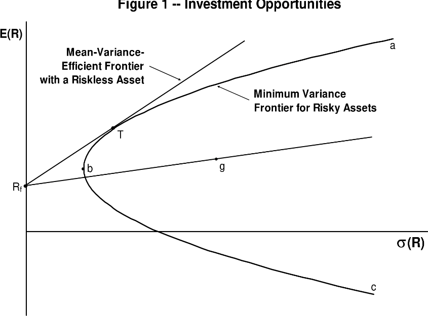
By comparing a stock’s risk and time value of money to its expected return, the CAPM formula establishes whether a stock is fairly valued. Building a portfolio with the CAPM is supposed to help investors manage risk (Perold, 2004). The efficient frontier is a curve that exists if a portfolio’s return were optimized perfectly by using the CAPM, which can be seen on the graph below.
Components of the CAPM
The CAPM comprises three components:
Expected return
The expected return is the loss or profit that an investor expects from foreign investment. The expected return is computed by multiplying the prospective outcome by the likelihood of their authoring it and adding the result.
Risk-Free Rate (Rf)
For starters, we can use the yield to maturity of default-free government bonds of equal maturity to each cash flow being discounted to find the risk-free rate (Chen, 2017).
Beta (β)
An equity’s beta represents its systematic risk compared with the broader market (i.e. nondiversifiable risk). An asset’s beta can be calculated as the variance of expected return on the asset minus the covariance between the asset and the market. Beta is often cited as a common cause of criticism of CAPM, since many view it as a flawed measure of risk.
Market Return
The model’s projected return is used to detect discounts to which is expected based on the capital appreciation and dividend of the stock for a specific holding or predicted period of time.
Market Risk Premium
The market risk premium is defined in the CAPM Model as the difference between the risk-free rate and the projected return on the market portfolio (Levy, 2018).
Expected Risk Premium (ERP)
Expected risk premium, the third input, refers to the incremental risk (or excess return) of investing in equity securities compared to risk-free securities.
Beta Calculations
Regression analysis is used to calculate beta. Essentially, it measures how quickly a security’s returns respond to changes in the market. Calculating beta involves dividing the variance of a benchmark’s return over a specific period by the covariance of an asset’s return over that benchmark.
A When assessing risk, it is important to consider a stock’s price variability. Beta has appeal as a proxy for risk if you think of it as the possibility that a stock will lose value. It makes sense intuitively. Furthermore, beta is a clear and quantifiable metric that is easy to work with (Magadi and Vutete, 2015). There certainly are variations in beta depending on factors such as the market index used and the measurement period. Yet broadly speaking, beta has a fairly simple definition. The cost of equity can be used to calculate the valuation method’s costs of equity. On Portfolio beta, on the other hand, is the average of the betas for each asset, according to their proportion in the portfolio. The portfolio beta is a measure of the relative volatility of a portfolio of securities based on the individual stock betas of securities in the portfolio.
Security Market Line (SML)
Security market lines (SML) serve as a visual representation of the capital asset pricing model (CAPM), which indicates the level of systematic risk that various marketable securities are exposed to, compared to the overall market’s expected return. An SML is also known as the “characteristic line,” which is a summary of the CAPM, with the x-axis representing risk (in terms of beta), and the y-axis representing return (in terms of expected return). Based on where a security is plotted on the chart relative to the SML, its market risk premium can be calculated. Both the CAPM and SML are based on the concept of beta. In the world of financial markets, the beta of a security represents its systematic risk, which cannot be eliminated by diversification. Market beta of one can be viewed as the average proportion of all securities (Bao, et al., 2018).
Results of an empirical test of the model
A beta value in excess of one indicates a risk level that is greater than the market average, and a beta value in excess of one indicates a risk level that is less than the market average.
Plotting the SML requires the following formula:
Required return = risk-free rate of return + beta (market return – risk-free rate of return)
FAMA-French 3 factor model
The transition from the CAPM model
The fundamental assumption behind this model as that value and small-cap stocks were able to outperform markets quite regularly. The model as essentially based an econometric regression of historical stock prices. The addition of value and size were able to explain the excess returns on stocks that could not be explained by the CAPM model (Basiewicz and Auret, 2010).
Historical background
The Fama and French Three-Factor Model (or the Fama French Model for short) is a pricing model that was developed in 1992. It was an extension of the CAPM model. The Fama Frech model expanded the CAPM model by also including the aspects of size risk and value risk factors to the established market risk factors.
The Three Factor model
According to this model, the expected rate of return is given as:
Where:
r = Expected rate of return
rf = Risk-free rate
ß = Factor’s coefficient (sensitivity)
(rm – rf ) = Market risk premium
SMB (Small Minus Big) = Historic excess returns of small-cap companies over large-cap companies
HML (High Minus Low) = Historic excess returns of value stocks (high book-to-price ratio) over growth stocks (low book-to-price ratio)
Now let us understand the components of the model:
Small Minus Big (SMB)
Small minus big (SMB) is a factor that says smaller companies outperform larger ones over the long-term and according to this model, this helps to explain the excess returns that small stocks gain in comparison to the big stocks. This also helps to contextualise the greater returns that investors can expect for investing into small stocks which are also associated with greater risks (Basiewicz and Auret, 2010).
In order to calculate SMB first we need to know the market capital of a company. Market capital is given as:
Now based on the market cap of the companies they are divided primarily into three broad categories: Large Cap (>$10 billion), Mid Cap ($2 billion to $10 billion) and Small Cap ($300 million to $2 billion). As the market capital increases, the risks are reduced and the prospective returns are also lower, generally. To calculate the SMB however, the stocks are sorted based on their market cap into five quintiles Q1 to Q5 where the bottom 20% of stocks, in terms of market cap, are placed in Q1 and to 20% of stocks are placed in Q5. Then the average returns in Q1 and Q5 are calculated and the difference in return between them is known as the SMB premium.
High Minus Low (HML)
High Minus Low (HML), also referred to as the value premium, accounts for the spread in returns between value stocks and growth stocks. The basic argument here is that companies with high book-to-market ratios, also known as value stocks, outperform those with lower book-to-market values, and are also known as growth stocks. This book to market value is calculated as the ratio between the accounting value of the company (assets – liabilities) and the market cap of the stock. Based on this B/M ratio as well the stocks are divided into 5 quintiles. The stocks in the top 20% B/M are placed in the value portfolio where as those in the bottom 20% are placed in the growth portfolio. The average returns then give us the HML premium’ (Cochrane, 2009).
Result of empirical test for the Three-Factor model
The model is mainly the outcome of economic reservations in previous stock prices, and size and value are seen as critical risk factors that aid in identifying and explaining the stock’s excess return.
FAMA-French 5 factor model
The FAMA-French 5 factor model is another extension of the FAMA-French 3 factor model which includes two new measurements into the valuation process. These include the RMW (Robust Minus Weak) and the CMA (Conservative Minus Aggressive) measures. The RMW measures the “Historic excess returns of stocks with robust profitability over stocks with weak profitability” where as the CMA measures the “Historic excess returns of stocks that invest conservatively and stocks that invest aggressively” (Chiah, et al., 2016)
Robust Minus Weak (RMW)
RMW is calculated based on the operating profitability of the stock. The operating profitability (OP) is, simply, the revenues minus cost of goods sold, minus selling, general, and administrative expenses, minus interest expense all divided by book equity. Here as well, stocks are segmented into 5 categories based on their OP here the top 20% are placed in the Robust portfolio while the bottom 20% are paced in the Weak portfolio. Similar to the other metrics the difference between the average returns in these two categories gives us the RMW premium.
Conservative Minus Aggressive (CMA)
To calculate the CMA we simply take the difference between the returns of firms with conservative and aggressive Investments. Here, we calculate the investment by the following formula:
Where is the change in assets from t-2 to t-1 and the is the total assets for the year .
As done before, the difference between average returns between the top quintile in terms of investment (Q1, Aggressive Portfolio) and the bottom quintile (Q5, Conservative portfolio) gives us the CMA premium.
The Carhart Four-Factor model
This model brings the momentum factor into calculating the value of the stock. This is done through the Winners Minus Losers (UMD) which is computed using cumulative historical returns in the previous 6 months or 1 year, and stocks are sorted according to this metric. The formula used in this model is:
The UMD premium in this case as well is determined by the difference in average returns of the top quintile stocks (Winners Portfolio, Q5) and the bottom quintile (Losers portfolio, Q1).
Conclusion
The preceding explanation can be used to identify the ultimate transition of the CAPM model to the three-factor model and eventually to the five-factor model. The many components and their application in the identification of the stock market and an organization’s investment are determined. The difference in the empirical test results for all models to indicate the excess return associated with stock management. The historical compliance of each model demonstrated the addition of other criteria that assist the investor more critically in determining the significance and greater appropriateness for investment. Aside from the parameters listed in the Asset price, other factors such as the bearing dimension of the sector and replicating the size of the portfolio might affect the Asset pricing. Apart from the inclusion of the five specified criteria, the magnitude of the profitability and Momentum can be used to estimate other parameters for the pricing model.
References
Bao, T., Diks, C. and Li, H., 2018. A generalized CAPM model with asymmetric power distributed errors with an application to portfolio construction. Economic Modelling, 68, pp.611-621. Available at: https://www.sciencedirect.com/science/article/pii/S0264999317304893 [Accessed on 22 February 2022].
Basiewicz, P.G. and Auret, C.J., 2010. Feasibility of the Fama and French three-factor model in explaining returns on the JSE. Investment Analysts Journal, 39(71), pp.13-25. Available at: https://www.tandfonline.com/doi/abs/10.1080/10293523.2010.11082516 [Accessed on 22 February 2022].
Chiah, M., Chai, D., Zhong, A. and Li, S., 2016. A Better Model? An empirical investigation of the Fama–French five‐factor model in Australia. International Review of Finance, 16(4), pp.595-638. Available at: https://onlinelibrary.wiley.com/doi/abs/10.1111/irfi.12099 [Accessed on 22 February 2022].
Cochrane, J.H., 2009. Asset pricing: Revised edition. Princeton university press.
Dimson, Elroy and R. A. Brealey. 1978. “The Risk Premium on UK Equities.” The Investment Analyst. December, 52, pp. 14–18.
Dionne, G., Li, J. and Okou, C., 2012. An extension of the consumption-based CAPM model. Available at SSRN 2018476. Available at: https://papers.ssrn.com/sol3/papers.cfm?abstract_id=2018476 [Accessed on 22 February 2022].
Fama, E.F. & French, K.R., 2004. The Capital Asset Pricing Model: Theory and evidence. Journal of Economic Perspectives, 18(3), pp.25–46.
Fama, E.F. and French, K.R., 2004. The capital asset pricing model: Theory and evidence. Journal of economic perspectives, 18(3), pp.25-46. Available at: https://www.aeaweb.org/articles?id=10.1257/0895330042162430 [Accessed on 22 February 2022].
Fisher, L. and J. H. Lorie. 1964. “Rates of Return on Investments in Common Stocks.” Journal of Business. January, 37, pp. 1–21.
Fisher, L. and J. H. Lorie. 1968. “Rates of Return on Investments in Common Stock: The Year-by-Year Record, 1926–1965.” Journal of Business. July, 41, pp. 291–316.
Gordon, Myron J. and Eli Shapiro. 1956. “Capital Equipment Analysis: The Required Rate of Profit.” Management Science. October, 3:1, pp. 102–10.
Levy, M., 2018. The continuous-time CAPM with non-risk-averse investors. SSRN Electronic Journal.
Markowitz, Harry. 1952. “Portfolio Selection.” Journal of Finance. March, 7, pp. 77–91.
Markowitz, Harry. 1959. Portfolio Selection: Efficient Diversifications of Investments. Cowles Foundation Monograph No. 16. New York: John Wiley & Sons, Inc.
Modigliani, Franco and Merton H. Miller. 1958. “The Cost of Capital, Corporation Finance, and the Theory of Investment.” American Economic Review. June, 48:3, pp. 261–97.
Perold, A.F., 2004. The Capital Asset Pricing Model. Journal of Economic Perspectives, 18(3), pp.3–24.
Roy, Andrew D. 1952. “Safety First and the Holding of Assets.” Econometrica. July, 20, pp. 431–39.
Savage, Leonard J. 1954. The Foundations of Statistics. New York: John Wiley & Sons, Inc.
von Neumann, John L. and Oskar Morgenstern. 1944. Theory of Games and Economic Behavior. Princeton, N.J.: Princeton University Press.
………………………………………………………………………………………………………………………..
Know more about UniqueSubmission’s other writing services:
