• Posted on August 2, 2022
• Libin

Assignment Sample on Economics and the Business Environment

Question 1

The makers of Porsche automobiles have adopted the slogan that states there is no substitute for Porsche. The cross-price elasticity of Porsche will be 0 if this is true as there is no substitute for the automobile. Consumers cannot shift to other items to rise in price for Porsche; the price elasticity of demand for Porsche will be very high.

Question 2

Prior to the outbreak of Corona Virus demand for hand sanitizers were not so inelastic, as it was not a necessary product (Oikarinen et al. 2018). After the outbreak, the product became highly necessary, and the demand for hand sanitizers of travel-size changed into highly inelastic. A sudden increase in demand exceeded the supply of hand sanitizers and caused shortages in the market. Street price for a hand sanitizer of travel-size rose from 0.99 GBP to 2.49 GBP.

Question 3

3. A. The sales of canned soda decreased by 2.5 as producers raised the price by 10 percent for canned soda from vending machines. For canned soda the elasticity of demand =

= -2.5/10

= 0.25

3. B. The change in the revenue percentage will depend on the percentage change in prices and demand. The fall in demand is greater than the rise in prices for canned soda, so the total revenue of the bottlers will fall after the change in price.

Question 4

4. A) The demand and supply equation for cod liver oil pills are, Qd = 100 – 4P, and Qs = -20 + 2P. At market equilibrium supply will equal demand.

Qd = Qs

100 – 4P = -20 + 2P

6P = 120

P = 20

For P=20, Q = -20 + 2*20

Q = 20

The equilibrium demand and price are 20, and 20 respectively.

4. b) At any price, the consumers want to acquire 60 bottles more, it will increase the price.

The changing demand for cod liver oil pills is (20 + 60) = 80.

80 = -20 + 2P

2P = 100

P = 50

The new price and quantity will be 50, and 80 respectively.

Question 5

The equilibrium quantity and price of good X were 5 million pounds and $10 in the previous year, which changed into 7 million pounds, and $12. Assuming the supply curve of product X is linear,

The change in producer surplus

= 0.5*(5+7)*(12-10) million

= 0.5*12*2

12 million

(B) Producer surplus changed from 12.5 million to 24.5 million

Question 6

6. a) Price elasticity of demand is -0.50 for a football match, and now prices are raised by 5 percent. The sold amount of ticket will be

= 5*(-0.5)

= -2.5

The number of tickets sold for football matches will lower off by 2.5 percent.

6.b) In the case of fried chicken, the elasticity of prices is -1.12 as it implies that the fall in the demand for fried chicken will be higher than the price increase. Overall expenditure on fried chicken will be lower as compared to earlier.

6. c) Demand for painkillers Qd = 1000 is given. The change in demand is zero for any change in prices due to a perfectly inelastic demand curve. At P = 100 GBP, the elasticity of demand will be zero.
7. d) The rise in the availability of substitute goods will increase the number of options for the consumers. As per the view of Lehner and Peer (2019), the increase in the level of the price will cause the customers to shift to another product. The elasticity of demand for the price will be higher as compared to earlier.
8. e) Reasons behind less elastic demand with respect to price are,
9. The substitutes are not available.
10. The items are necessary for nature.

Question 7

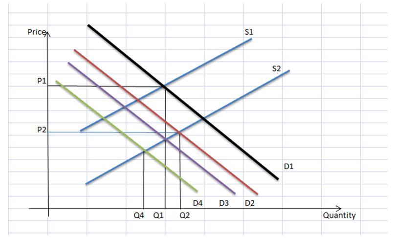
Figure 1: Market Equilibrium for Lobster

(Source: Created by Learner)

The fall in the income of the consumer declined the demand for lobsters whereas a record harvest of lobsters created a massive supply in the market. Lower demand for the lobster decreased the level of demand for lobster as well the prices. The massive supply of lobster shifted the supply curve to the right, and further lowered the price which increases the level of demand. The equilibrium quantity of the lobster will depend on the change in the extent of the shift of the supply curve and demand curve. The size of the change in demand or supply cannot be identified; hence the equilibrium level of the amount cannot be estimated.

(2) The equilibrium amount cannot be predicted but the equilibrium level of the price will fall.

Question 8

8. a) The subsidy size = (10-6)

= 4

8. b) The level of prices paid by the customers after, and before the subsidy are $6, and $8.
9. c) The level of prices received by the producers after, and before the subsidy is $10, and $8.
10. d) The amount of consumer abundance before subsidy

= 0.5*(16-8)*4

= 0.5*8*4

= 16

The amount of consumer abundance after subsidy

= 0.5*(16-6)*5

= 0.5*10*5

= 25

8. e) The amount of producer abundance before subsidy

= 0.5*8*4

= 16

The amount of producer abundance after subsidy

= 0.5*10*5

= 25

8. f) The subsidy cost of the government

= 5*(10-6)

= 20

8. g) The amount of deadweight loss for this subsidy

= 20 – [(25-16) + (25-16)]

= 20 – 18

= 2

Question 9

9. a) In the free market the equilibrium level of price, and amount are respectively $8.52, and 330 box per week.
10. b) Mow, there is a quota on boxes of ammunition that is imposed at 200, and the new equilibrium level of the amount is 200. The level of the price will be derived from the demand curve, and it is estimated at $12.
11. c) A, B, and E letters depict the amount of consumer surplus preceding the quota.
12. d) C, D, and F letters depict the amount of producer surplus following the quota.
13. e) A depicts the amount of consumer surplus preceding the quota.
14. f) B, C, and D letters depict the amount of producer surplus following the quota.
15. g) E, and F depict the amount of deadweight loss from the quota.

Question 10

10. A. Demand, and supply equation for almonds in the market are Qd = 80 – 10P, and Qs = 10P

80 -10P = 10P

20P = 80

P = 4

At equilibrium level of amount = 80 – 10*4

Q = 40, where Q measures in hundreds of bags per day.

10. B. Level of consumer abundance = 0.5(80 – 40)*4

= 0.5*40*4

= 80 hundred

Level of producer abundance = 0.5*40*4

= 80 hundred

10. C. The price floor is imposed at $7, which is higher than the equilibrium price at the free market. The price floor will increase the level of supply as well a decline in demand, and an abundance of almonds will happen in the market.

Level of supply at $7, Qs = 10*7

Qs = 70

Level of demand, Qd = 80 – 10*7

Qd = 10

Size of the abundance = 70-10

= 60

10. D. Consumer abundance with price floor = 0.5*(8-7)*10

= 5 hundreds

Producer abundance with price floor = 0.5(7+6)*10

= 65 hundreds

10. E. Deadweight loss size = (80 + 80) – (5 + 65)

= 160 – 70

90

Question 11

The demand for the items is depicted by D1 in the short-run, and from a point, the price-quantity adjustment process is initiated. The consumer makes decisions based on the price level of the current period, whereas the producer supplies the number of items considering the price of the preceding period. In the short-run, the adjustment process follows the price mechanism and gradually converges to the level of equilibrium (Calvert Jump, 2018). The supply and demand for the items will change into an equilibrium level of P*Q*.

In the long-run all factors of production are variable, and producers can incorporate all the factor cost in the production. The long-run demand curve for the good is depicted by D2, and the price-quantity adjustment process initiated from point a’. As per the view of Albagli et al. (2019), the suppliers can estimate the behaviour of the customers as well can identify the cost of production

Question 12

The initial demand line and supply line was denoted by AB, and GH and equilibrium is depicted at E. A subsidy was given on the sales of wine resulting in the rise of an equilibrium amount of wine from Qe to Qs. In the new scenario, the price received by the consumer is Ps per unit, and the price paid by the customers is Pc per unit.

12. a) The cost of the subsidy is depicted by the area PsSCPc.
13. b) Social welfare depends on the level of consumer abundance, and producer abundance (Lam and Liu, 2017). The gain in consumer abundance is the area PeECPc, and the gain in producer abundance is the area PeESPs. However, the total gain in producer and consumer abundance is offset by the cost of subsidy as subsidy produces a deadweight loss. The area of ECS denotes the deadweight loss and it decreases the level of social welfare.

Question 13

The sales tax imposed by the government is referred to as the imposition tax on the sale of any or particular services or items. As per the view of Brunner and Schwegman (2017), the sales tax raises the level of price of commodities and services. The price value of the products increases along with a fall in demand for the product and the equilibrium price will fall. The demand for liquor is more inelastic as compared to the demand for rental video. The changes in the demand depend on the elasticity for prices as higher elastic demand causes more shifts in demand for any service or product (Cabello et al. 2020). The tax burden will fall more on the owner of a local rental video store than the owner of a local liquor store. Hence, the owner of a local video rental store will object to the proposed idea of a 1 percentage increase in city sales tax.

Question 14

A tariff is a tool that obstructs free trade in the international markets as it protects domestic suppliers from cheap imported foreign items. Tariffs increase the prices of the items, and domestic suppliers wish to produce the item to a greater extent. As per the view of McCausland et al. (2020), tariff reduces the overall import level, raises the level of production.

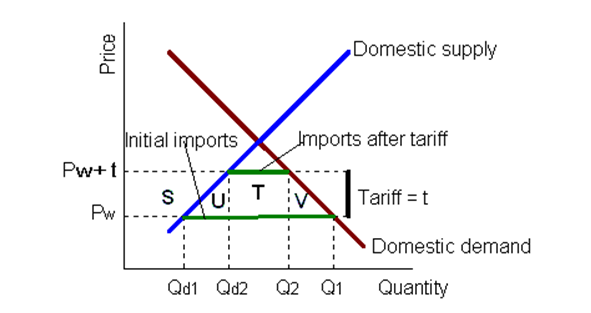
Figure 2: Tariff on Domestic Economy

(Source: Chekh and Semiv, 2017)

In this scenario, tariffs increased the price of imported products from Pw to domestic price level Pt. The welfare of the domestic customers reduces significantly as they have to buy the item at higher prices. The consumer abundance that can be depicted as the area U, T, and V was earlier beneficial to customers but the imposition of tariff seizes the surplus. The domestic suppliers of the items are benefited due to the imposition of tariff and gain in their producer surplus can be depicted by area U.

The government of the domestic nation gets benefited as they earn the tariff amount from consumers as their revenue. The revenue generated by the government can be depicted by area T. From the viewpoint of Lam and Liu (2017), the overall level of social welfare of a nation depends on the total consumer abundance, supplier abundance, and government welfare. The domestic economy has a negative effect as a deadweight loss is generated due to the imposition of the tariff, and net loss can be depicted by area T.

Question 15

15. a)

Quantity	Total Revenue	Fixed Cost	Variable Cost	Total Cost	Profit = Revenue – Total Cost	Marginal Revenue	Marginal Cost
0	0	10				—	—
1	18	10	8	18	0	0	8
2	36	10	4	22	14	14	12
3	54	10	6	28	26	12	18
4	72	10	9	37	35	9	27
5	90	10	12	49	41	6	39
6	108	10	13	62	46	5	52

 

Table 1: Profit-maximizing table of Emma

(Source: Created by Learner)

15. b) The production output of Emma will be 4 shawls per week.
16. c) The marginal cost will be the same as the marginal revenue at the point where profit maximizes (Hottenrott et al. 2017).
17. d) Emma’s fixed cost for producing shawls falls to 7 GBP.

Quantity	Total Revenue	Fixed Cost	Variable Cost	Total Cost	Profit = Revenue – Total Cost	Marginal Revenue	Marginal Cost
0	0	7				—	—
1	18	7	8	15	3	3	8
2	36	7	4	19	15	12	12
3	54	7	6	25	29	14	18
4	72	7	9	34	38	9	27
5	90	7	12	46	44	6	39
6	108	7	13	59	49	5	52

Table 2: New Profit-maximizing table of Emma

(Source: Created by Learner)

Reference List

Albagli, E., Fornero, J., Fuentes, M. and Zúñiga, R., 2019. On the effects of confidence and uncertainty on aggregate demand: evidence from Chile. Economía chilena, vol. 22, no. 3.

Brunner, E.J. and Schwegman, D.J., 2017. The impact of Georgia’s education special purpose local option sales tax on the fiscal behavior of local school districts. National Tax Journal, 70(2), pp.295-328.

Cabello, O.G., de Moraes, G.H.S.M., Watrin, C., da Silva, H.M.R. and Spers, E.E., 2020. The Influence of Sales Tax Transparency and Political Trust on Brazilian Consumer Behaviour. Journal of Accounting, Management and Governance, 23(1), pp.141-161.

Calvert Jump, R., 2018. Inequality and Aggregate Demand in the IS‐LM and IS‐MP Models. Bulletin of Economic Research, 70(3), pp.269-276.

Chekh, M. and Semiv, G., 2017. Shocks of the aggregate demand and balance of payment equilibrium in a dependent economy. Economic annals-XXI, (163), pp.47-51.

Díaz, A.O. and Medlock, K.B., 2021. Price elasticity of demand for fuels by income level in Mexican households. Energy Policy, 151, p.112132.

Dolšak, J., Hrovatin, N. and Zorić, J., 2020. Factors impacting energy-efficient retrofits in the residential sector: The effectiveness of the Slovenian subsidy program. Energy and Buildings, 229, p.110501.

Goyal, A. and Kumar, A., 2018. Active monetary policy and the slowdown: Evidence from DSGE based Indian aggregate demand and supply. The Journal of Economic Asymmetries, 17, pp.21-40.

Hottenrott, H., Lopes-Bento, C. and Veugelers, R., 2017. Direct and cross scheme effects in a research and development subsidy program. Research Policy, 46(6), pp.1118-1132.

Lam, C.T. and Liu, M., 2017. Demand and consumer surplus in the on-demand economy: the case of ride sharing. Social Science Electronic Publishing, 17(8), pp.376-388.

Lehner, S. and Peer, S., 2019. The price elasticity of parking: a meta-analysis. Transportation Research Part A: Policy and Practice, 121, pp.177-191.

McCausland, W.D., Summerfield, F. and Theodossiou, I., 2020. The Effect of Industry-Level Aggregate Demand on Earnings: Evidence from the US. Journal of Labor Research, 41(1), pp.102-127.

Mierau, J.O. and Mink, M., 2018. A descriptive model of banking and aggregate demand. De Economist, 166(2), pp.207-237.

Oikarinen, E., Bourassa, S.C., Hoesli, M. and Engblom, J., 2018. US metropolitan house price dynamics. Journal of Urban Economics, 105, pp.54-69.

 Assignment Services Unique Submission Offers: