
Module Code : CIS7031 Employment in Wales
WRIT 1
1.1 Downloaded dataset of Wales total employment valu
| Industry | 2018 | 2017 | 2016 | 2015 | 2014 | 2013 | 2012 | 2011 | 2010 | 2009 |
| Agriculture | 41100 | 40200 | 43200 | 40700 | 42700 | 36800 | 36100 | 36100 | 38200 | 37700 |
| Production | 165700 | 165100 | 162500 | 172300 | 173300 | 164200 | 154400 | 158600 | 149800 | 156700 |
| Construction | 101800 | 90800 | 102700 | 92600 | 97000 | 89300 | 91300 | 90000 | 93200 | 96600 |
| Retail | 190600 | 185100 | 198400 | 206700 | 194300 | 200900 | 202800 | 202600 | 202700 | 203700 |
| ICT | 31500 | 58900 | 34400 | 24000 | 35700 | 26900 | 27200 | 26400 | 27900 | 27800 |
| Finance | 35500 | 32100 | 31000 | 30800 | 32400 | 32400 | 31100 | 33200 | 29800 | 33800 |
| Real_Estate | 25200 | 18200 | 22700 | 19100 | 22200 | 18000 | 18800 | 17600 | 14600 | 13500 |
| Professional_Service | 89000 | 82300 | 72000 | 78500 | 64800 | 72500 | 59100 | 63900 | 64000 | 64100 |
| Public_Adminstration | 89600 | 86000 | 83200 | 85600 | 86700 | 89500 | 88100 | 88700 | 93100 | 92800 |
| Other_Service | 81800 | 83200 | 72400 | 77200 | 73300 | 75500 | 72800 | 72400 | 68000 | 64200 |

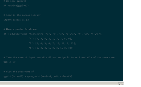
Sample code to create a datafram is given below
1.2 Check for any null value or outlier.
The data points that are far from the data points are called outliers. Outliers are unusual values in the given dataset which are problematic in statistical analyses which may cause miss significant findings or distort real results.
No definite statistical rules are available for identifying these outliers it depends upon the knowledge of the subject and the understanding of the collected data process.
There are some guide lines for the statistical test for finding the outlier. Outliers are notably different from all the data collected. There are many methods to find the outliers in the given data set which are categorised into visual and analytical assessments. Sorting the datasheet is one of the simple and effective ways to find out the unusual values.
Boxplots, histograms and scatterplots are also used to find out the outliers. Boxplots display any symbols or asterisk on the graph to indicate the outliers in the datasets. It uses the inter quartile method to find the outliers. It can also be used to find the outliers in the group of the data. Histograms help to emphasize the outlier by isolated bars.
Scatterplots can also used to detect outliers in multivariate variables. A scatterplot along with the regression line is used to find out the points that are followed to the line and the points that are away from the line are outliers. Hypothesis tests can be used to find out the outliers.
Z-scores are also used to find the outliers which are used to quantify the unusualness of an observation when the data follow a normal distribution. It is the number of standard deviation of the each value. When the values are equal to the mean then the Z-score value will be represented by zero.
The outliers can also be found out using the inter quartile range (IQR). There are no null values found in the data set.
Check for finding outlier is done by calculating the 1st Quartile (Q1) and 3rd Quartile (Q3) and based on the value obtained IQR (Inter Quartile Range) is calculated. Upper bound is set using the formula Q3 + (1.5*IQR) and the lower bound is calculated using the formula Q1 – (1.5*IQR).
Outlier is identified by comparing the given value with the upper bound and the lower bound. It the given value is greater than the upper bound and less than the lower bound the data is set to be an outlier. In the given dataset no outlier are found.
| Industry | 2018 | 2017 | 2016 | 2015 | 2014 | 2013 | 2012 | 2011 | 2010 | 2009 |
| Agriculture | 41100 | 40200 | 43200 | 40700 | 42700 | 36800 | 36100 | 36100 | 38200 | 37700 |
| Production | 165700 | 165100 | 162500 | 172300 | 173300 | 164200 | 154400 | 158600 | 149800 | 156700 |
| Construction | 101800 | 90800 | 102700 | 92600 | 97000 | 89300 | 91300 | 90000 | 93200 | 96600 |
| Retail | 190600 | 185100 | 198400 | 206700 | 194300 | 200900 | 202800 | 202600 | 202700 | 203700 |
| ICT | 31500 | 58900 | 34400 | 24000 | 35700 | 26900 | 27200 | 26400 | 27900 | 27800 |
| Finance | 35500 | 32100 | 31000 | 30800 | 32400 | 32400 | 31100 | 33200 | 29800 | 33800 |
| Real_Estate | 25200 | 18200 | 22700 | 19100 | 22200 | 18000 | 18800 | 17600 | 14600 | 13500 |
| Professional_Service | 89000 | 82300 | 72000 | 78500 | 64800 | 72500 | 59100 | 63900 | 64000 | 64100 |
| Public_Adminstration | 89600 | 86000 | 83200 | 85600 | 86700 | 89500 | 88100 | 88700 | 93100 | 92800 |
| Other_Service | 81800 | 83200 | 72400 | 77200 | 73300 | 75500 | 72800 | 72400 | 68000 | 64200 |
2.1 Highest and lowest workers
Retail industry has employed highest workers and real estate employed the lowest workers over the period of 2009 to 2018. The graph shows depicts the dataset of Wales employment.
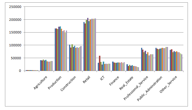
2.2. Highest and lowest overall growth
Retail industry has the highest growth and the real estate have a lowest growth. The graph shown in 2.1 supports the answer.
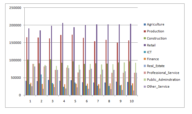
2.3 Best and worst performing year
Year 2018 is the best performing year and 2013 is the worst performing year in relation to number of employment.
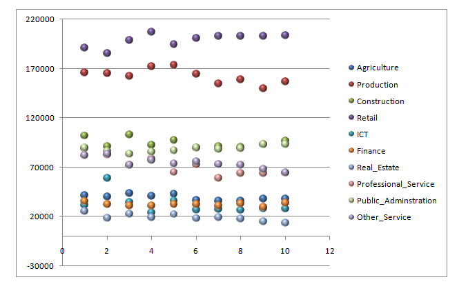
Create a dynamic scatter/bubble plot showing the change of workforce number over the period using
Average employment number for each industry over the period
| Industry | Average employment number |
| Agriculture | 39280 |
| Production | 162260 |
| Construction | 94530 |
| Retail | 198780 |
| ICT | 32070 |
| Finance | 32210 |
| Real_Estate | 18990 |
| Professional_Service | 71020 |
| Public_Adminstration | 88330 |
| Other_Service | 74080 |
Retail industry is the highest correlated industry while real estate is the lowest correlated industries.
4.2 Year wise correlation for each industry
| 2018 | 2017 | 2016 | 2015 | 2014 | 2013 | 2012 | 2011 | 2010 | 2009 | |
| Agriculture | 1 | |||||||||
| Production | 0.982563 | 1 | ||||||||
| Construction | 0.992946 | 0.982398 | 1 | |||||||
| Retail | 0.99622 | 0.982002 | 0.995812 | 1 | ||||||
| ICT | 0.988976 | 0.984139 | 0.996273 | 0.994068 | 1 | |||||
| Finance | 0.994441 | 0.983212 | 0.995358 | 0.998684 | 0.994628 | 1 | ||||
| Real_Estate | 0.985425 | 0.974904 | 0.994625 | 0.992952 | 0.992828 | 0.996405 | 1 | |||
| Professional_Service | 0.989176 | 0.978012 | 0.995347 | 0.995818 | 0.994201 | 0.998576 | 0.999355 | 1 | ||
| Public_Adminstration | 0.985296 | 0.973743 | 0.993573 | 0.990992 | 0.989227 | 0.99502 | 0.998115 | 0.997776 | 1 | |
| Other_Service | 0.986112 | 0.973968 | 0.994785 | 0.991446 | 0.991894 | 0.995055 | 0.997301 | 0.997702 | 0.998922 | 1 |
Yes all the industries are correlated over each year except the retail industry where the correlation value of the retail industry is very low during the year 2018 when compared with other industries. All other industries have only a slight variation in the correlation values over the years.
5. Clustering (k means & hierarchical)
K means is used to find the local maxima using iterative clustering algorithm. In the first step k is taken as 2. Random points are assigned to each point in the cluster. Then the centroid point for the cluster is selected using a different colour. Closest cluster centroids are re-assigned.
Cluster centroids are recomputed for the entire cluster. The cluster is formed by taking k value as 3 and the cluster is formed between the clusters of the successive points and the steps are repeated until there is now switching of data between two clusters which marks the termination of the k means algorithm.
It is one of the most common testing techniques used in Machine Learning. Hierarchical clustering is divided into two types Agglomerative and Divisive. In agglomerative each data point is considered as an individual cluster and merges the similar cluster during each iteration and the clustering is done until one or K clusters are formed.
The Agglomerative algorithm is straight forward it computes the proximity matrix and each point is considered as a cluster, the process of merging the two closest clusters is done and it is updated in the proximity matrix this process is repeat until a single cluster remains.
Computation of the proximity of two clusters is the key operation of this algorithm. Hierarchical clustering can be visualized using a Dendrogram it is a tree-like structure diagram that which records the sequences of merge and splits in the data.
It is the most common used clustering technique while Divisive hierarchical clustering is not commonly used. It is opposite to the Agglomerative clustering. In this method all the points are considered as a single cluster during each iteration the data that are not similar are separated from the cluster.
Such separated points are considered as an individual cluster. The single cluster is divided into n clusters in the Divisive hierarchical clustering. Hierarchical clustering algorithm builds the cluster hierarchy.
In hierarchical cluster consider all the data points in the data set and form its own cluster. Two nearest clusters are merged into one cluster this will continue until a single cluster is framed. In k means cluster we will a mean value for cluster and frame the cluster.
Hierarchical cluster cannot be used for big data while K means cluster is best suited for big data. The time complexity of K means is linear O(n) while hierarchical clustering is O(n2). K means a random choice is made to choose the cluster.

.The employment landscape of Wales was constantly increasing in all the fields constantly during all the years. In the year there is only a slight variation among the industries based on the employments made. Different type of analysis is made on the data.
The data is first collected from the website and data frame is formed. Analysis is made to find if there is any outliers in the data set by calculating the first quartile and the third quartile of the date then the inter mediate quartile is framed upper and lower bound of the data for each industry is set and compared with the data frame to find out the outliers.
A visual analysis is made on the data frame by creating a bubble scatter chart using plotly which shows that all the clusters are close to each other. Then a correlation was created on the data for every product over the year.
By analysing the correlation we can find that all the correlation values are mostly same except one value of the Retail industry during the year 2018.
Then using the same data set K means clustering and hierarchal clustering algorithms are applied and clusters are framed in K means by keeping the k value as 2 in the first iteration and a second iteration is done with the k value 3 where clusters framed during the two iterations are almost same.
Then a hierarchal cluster algorithm is applied for the same data set which takes all the data in the data set and clusters are framed.
The final result show that the employment landscape of the Wales is constantly increasing over the period of time without more deviation in all the industry. Different analysis made on the data set confirms that the employment of the Wales is gradually increasing without any deviation throughout the years for all the 10 industries.
- O. Omolehin, A. O. Enikuomehin, R. G. Jimoh and K. Rauf, (2009) “Profile of conjugate gradient method algorithm on the performance appraisal for a fuzzy system,” African Journal of Mathematics and Computer Science Research,” vol. 2(3), pp. 030-037.
- V. Anand Kumar and G. V. Uma, (2009) “Improving Academic Performance of Students by Applying Data Mining Technique,” European Journal of Scientific Research, vol. 34(4).
Azar, A., Sebt, M. V., Ahmadi, P., & Rajaeian, A., (2013) “A Model for Personnel Selection with A Data Mining Approach: A Case Study in A Commercial Bank: Original Research”. SA Journal of Human Resource Management, 11(1), 1-10.
Al-Radaideh, Q. A., & Al Nagi, E., (2012) “Using Data Mining Techniques to Build a Classification Model for Predicting Employees Performance”. International Journal of Advanced Computer Science and Applications, 3(2).
Lakshmi, T. M., Martin, A., Begum, R. M., & Venkatesan, V. P. (2013) “An Analysis on Performance of Decision Tree Algorithms using Student’s Qualitative Data”. International Journal of Modern Education and Computer Science, 5(5), 18.
Priyama, A., Abhijeeta, R. G., Ratheeb, A., & Srivastavab, S. (2013) “Comparative analysis of decision tree classification algorithms”. International Journal of Current Engineering and Technology, 3(2), 334-337.
Ronald E. Shiffler (1988) Maximum Z Scores and Outliers, The American Statistician, 42:1, 79-80,
