Finance for International Business

Introduction

In the year 1970, Fenland Foods plc. was established when an arable farm was acquired by Williams familyin Lincolnshire. Even though the business was increased rapidly it remained a family business. Later in the year 1980 it was restructured as a company. In the year 1991, directors of the company determined that the business present form was at its highest development limit. Therefore, there was a need for business expansion so as to create a competitive advantage. Several possibilities were investigated by them to expand the business later they set up their system of distribution. With the expansion of the business new and innovative production technology was implemented by the directors.

Methodology

WACC (weighted average capital cost)

The finance director anticipates that there will be a new venture to achieve the current return on capital and this venture will break even within a period of not more than five years. The project, which is biased towards expanding the business, requires that the company purchase 1,000 acres of land in the Republic of Ireland. The company will also have to invest in agricultural machinery, which will be depreciated 10% annually on a straight line method of reduction. Estimated cash flows are calculated in Euro currency. The capital budgeting strategies used to evaluate project realities are nominal repayment periods, NPVs, and IRRs.

It is important to consider the performance of the company in the last two financial years as it will help determine the profitability position, liquidity, efficiency and flexibility of the company or level of financial risk. The company’s performance has been evaluated in 2020, using profitability, liquidity, efficiency and transparency ratios (Müllner, 2017).

Present value (PV)

Present value (PV) is the current value of the future amount of cash or the steam of cash flows provided a stated rate of return. There will be discounts with higher rates of cash flows and higher discount rates, which will be lower in future cash flows. Moreover, measuring the appropriate discount rate is the key to forecasting future cash flows, be it income or liability.

Net Present Value

NPV measures the profitability of the project. It shows the amount of income from the project after deducting the initial cost. NPV can be positive, zero or negative. Positive current value results when the project has a higher current cash flow than the initial cost. It should be accepted if the NPV of the project is positive. Zero net present value results when the current value of a project’s cash flow is equal to the initial cost. Investment may or may not be acceptable if NPV is zero. The negative NPV results when the project’s initial cost estimate is higher than the discounted cash flow. If it has a negative NPV, the expansion should not be performed.

The required rate of return is determined using CAPM; It is used as a discount rate. From the spreadsheet calculation, the project’s NPV at a discount rate of 9.01% is negative. Thus, the organization should not accept the project (Esty, 2014).

Internal Return Rate (IRR)

The IRR is the minimum discount rate used to measure the project’s ability to achieve return. This is the result of zero NPV. A project with an IRR greater than or equal to the discount rate should be rejected otherwise. The company’s IRR is 8.93% lower than the discount rate. Thus, the organization should not do the project because its IRR is no better than the discount rate.

Payback period

There is a nominal repayment period for the project’s cash flow to recover the initial investment cost. Initial investment should only be considered if it promises to take less time to recover the initial cost. The project should be adopted that is equal to or less than the maximum desired payback period for the payback period management. The finance director wants the longest payback period for five years while the calculated payback period is 7.7 years. The calculated payback period is longer than the manageable payback period. Therefore, the project should not be undertaken on the basis of this strategy.

Result

The option is the purchase of the organization at £1,500,000. It is expected that the organization will be sold €870k in 2021 as well as grow at 12% per annum to 2025. This shows that the average investment through the period will be £1,500,000.

ARR = 20.83%

The cumulative cash flows turn positive for the primary time in 5 years.

Payback period = 5.68 years.

The NPV is £738,000

IRR is 19.44%.

Implications of Results: Viability of The Project

The ARR is 20.83%. There are no criteria accessible for assessment, but these are higher than the cost of capital expenditure of 12%. Therefore, the ARR method allows investment. Moreover, the payback period to be 5.68 years. Although the payback period is shorter than the10-year life of the project, it doesn’t meet the 5-year cut-off period for the finance manager. Thus, the investment is not allowed under the payback period method

Then again, NPV is very high and positive £738,000. Buying of the organization will increase the firm’s net worth by $ 738,000 over a 10-year period. Therefore, the investment under the NPV method is approved. At last, the IRR of 19.43% is similarly higher than the cost of capital of 12% that another time approves the purchase of the organization(PierdziochRisse&Rohloff, 2014).

In addition to the above analysis, there are a few other important things to keep in mind when making investment decisions. First, it is estimated that the company will sell for $ 1,500,000 after 10 years. However, in the last one year, the costs of farm and land continued to rise.

The annual company price inflation of 6% over a ten-year period, which might rise NPV to £1,121,000. This is an important jump. Despite the annual company price inflation is (-2%), NPV is still positive. Then again, the significant benefits from buying organization should also include final decision making.

Second, prices are also complex to changes in flow. The practice is rarely seen in practice. This is hard to forecast cash flows through a 10-year period due to several factors. Moreover, the demand can change as the economy changes. Besides, the cost of raw materials and labor may increase more rapidly than expected. Thus, it is useful for analyzing cash flow sensitivity. It is possible that there will be a direct proportion to the change in the income of variable costs.

In addition to the points discussed above, the organization needs to analyze a few major non-financial factors to confirm that this investment will make positive outcomes. Moreover, the purchasing power of buyers is associated with general economic circumstances. The economy of the UK is crossing in a difficult phase with customer concerned about the government cut in the public expenditure. It can make it problematic for the organization to sell products in the local area.

Financing Options

Solvency ratio

Solvency Ratios	2019	2020	Average
Debt Ratio	0.36	0.36	0.36
Debt to Equity Ratio	0.56	0.57	0.57
Times Interest Earned	16.38	12.40	14.39

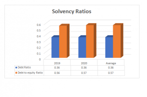
Debt Ratio

The debt ratio shows the level of financial risk the company is exposed to; the higher the ratio the higher the financial risk. Company stakeholders use this ratio to measure the company level of financial risk. The debt ratio in both years is 0.36. The optimal debt ratio is 0.50. the debt ratio for the past 2 years is below 0.5: this indicates that the company was less geared. The company is having more assets than liabilities, only 36% of the company capital is made up of liabilities. Moreover, creditors own the firm with a less percentage than asset holders. The company’s financial risk is low due to high equity in its capital structure. In addition, the organization still operates under going concern supposition since it has more assets to operate after it has paid all its debts. Creditors of the company use this ratio to determine the company’s ability to pay. The Organic Farm Foods plc is most likely to be considered by a bank for loans since it has low debt, hence a minimal risk of default (Verbeke, 2013).

Debt-to-equity ratio

The debt-to-equity ratio measures the weight of debt in the company capital structure. The optimal ratio for debt to equity is 0.5. the ratio greater than 0.5 means that the capital structure is made of more debt than equity. The debt-to-equity ratio increased to 0.57 in 2020 from 0.56 in 2015; this shows an increase in the gearing level o0f the company. The average Debt-to-equity ratio for the two years is 0.57. The ratio is above 0.5 in the two years; therefore, the company has more equity than debt in its capital structure.

Times Interest Earned or Interest Cover

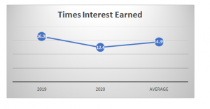
Times Interest Earned ratio measures the capability of the organization to pay its future interest expense without a doubt. The interest cover ratio of the company is very high. It means that the organization is much able to pay interest on outstanding loans. Operating income generated is sufficient enough to cover the future interest expense. The ratio is considered by both investors and creditors. Creditors consider a higher ratio when approving loans to firms. The company is eligible for a loan because its interest cover ratio is very high (Hamilton & Webster 2018).

Value creation

Liquidity Ratios

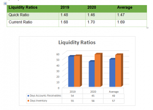
Quick Ratio

The ratio measures the percentage of current liabilities a company can pay off when fall due using quick assets. In addition, the optimal quick ratio is 1at a ratio of 1. Also, the organization can settle 100% of its current liabilities by quick assets. Further, the ratio of the organization in 2019 is 1.43. It shows quick assets are sufficient to settle the current obligations. The ratio has decreased in 2020 to 1.46 due to an increase in stock and other short-term liabilities. There is a prospect that the organization sold its fixed assets to compensate for the remaining percentage of current liabilities that the organization could not furnish for using quick assets. The average ratio is to 1.47, this shows a higher liquidity position for the previous years. Total current assets fewer inventories were almost 1.5 times current liabilities. The fluctuation in quick ratio means that the liquidity of the company fluctuates year after the year (Kaynak& Baker, 2013).

Current Ratio

The ratio measures the capability of the organization to compensate its current liabilities by means of current assets. Also, the optimal current ratio is 1; the ratio at which current assets are equal to current liabilities. The ratio of the company in 2019 is 1.48; current assets can be used to pay off current debts fully. The ratio has increased to 1.70 in 2020 due to a decrease in short-term loan and the overall decrease in current liabilities; current assets were almost twice current liabilities, the company still remained with 70% of the assets after fully paying off current liabilities. There was no requirement for the organization to sell its fixed assets to pay off the current debts. The average ratio of 1.69, this shows that the company is more liquid. Total current assets were almost twice the current liabilities. Moreover, the organization was able to pay off its current liabilities in full and remain with more than half of current assets. In this way, the company is more liquid as the current ratio is higher(Kaynak& Baker, 2013). The average ratio is more than 1 andit shows that the company is liquid.

Efficiency Ratio

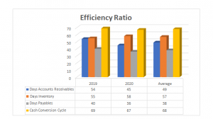
Efficiency Ratios	2019	2020	Average
Days Accounts Receivables	54	45	49
Days Inventory	55	58	57
Days Payables	40	36	38
Cash Conversion Cycle	69	67	68

Days receivable outstanding

Days receivable outstanding measures the period is taken by the company to collect cash from its debtors, usually 30 days. Debtors collection period decreased in 2020. 2020 bears the lowest ratio; this indicates that the company changed its credit policy to favor a shorter collection period; the shorter the cash collection period the more improved the cash flows are. The company should consider having the shortest possible cash collection period so as to avoid the risk of the time value of money. The average collection period is 49 days; this is longer than the optimal collection period of 30 days. The company should tighten its credit policy so as to reduce the number of days covered to collect cash from its customers (Cuervo-Cazurra, 2016).

Days Payables outstanding

Days payable outstanding is the period covered by the company to pay its suppliers. The duration covered depends on how the company negotiates with its suppliers. A company with a more extended average creditor period has an improved cash flow; however, creditors might not be happy. The Days payable outstanding decreased to 36 in 2020 from 40 in 2019; this indicates that the company took a shorter to pay off its creditors in 2020 than in 2019. The cash flow of the company is improved with the longer days payable outstanding. The average days payable outstanding is 38; this shows that the company is more active in considering creditor’s payment, it does not wait until it collects all the outstanding receivable to pay its creditors. An optimal average inventory period is 30 days. Therefore, a high ratio helps improve the company cash flow; however, creditors might not be happy.

Days inventory outstanding

Days inventory outstanding is the period covered by inventory in store before they are sold off. The Days inventory outstanding increased in 2020; this indicates that the company took longer to clear off its stock in 2020 than 2019. The shorter period shows how efficient the company management is in selling the company products. An optimal average inventory period is 30 days. The average days’ inventory outstanding is 57days. Days inventory outstanding is longer. Therefore, the company should carry out a successful advertisement of its products in order to increase sales (Stadelmann, Michaelowa& Roberts, 2013).

Cash Conversion Cycle (CCC)

The ratio measures the efficiency of the company in buying, selling, and collecting cash from its customers; The higher the ratio the more efficient the company is. CCC of the company is determined to subtract the average creditor’s payment period from the sum of the average inventory selling period and average debtors collection period. The cash conversion cycle gradually decreased from 69 days to 67 days. The higher the cash conversion the more active the company is. therefore, it means that the company was more active in 2020 than in the previous period. The lower cash conversion cycle attained in 2020 shows that the company’s money was held in its inventories for a shorter period. The company is able to buy, sell and collect cash from its customers within a shorter period.

Exchange Rate Volatility

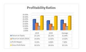
Profitability ratio

Profitability Ratios	2019	2020	Average
Return on Equity	23.13%	20.15%	21.64%
Return on Assets (ROA)	14.83%	12.81%	13.82%
Profit Margin	8.24%	6.96%	7.60%
Gross Profit Ratio	30.51%	29.91%	30.21%

Return on Equity

Return on equity decreases from 2019 all through to 2020; this implies that the rate at which shareholders’ equity is utilized to generate income has decreased in 2020 as compared to the previous year. The company managed to generate $0.23 for every coin of equity spent in 2019, and this decreased to $0.20 return generated in 2020 from every dollar of the equity fund. Moreover, the average amount of return on equity generated for the three years is $0.22. A high return on the company’s equity shows the effective management of shareholders’ funds. In addition, the return restored per equity fund is the higher and the management of the company is more effective. The ratio shows that the management is committed to maximizing the company profits hence maximizing the shareholder’s value. Based on return on equity, the company is more profitable and good for the client. Every investor prefers a firm with a high return on equity than the one with a low ratio. Calculation of the company’s equity allows the owners to ascertain the profitability performance of the company as well as its ability to maintain the high trends in income (Hillier, et al. 2014).

Return on Assets

Return on assets decreased from 14.83% in 2019 to 12.81% in 2020: this implies that the amount of income generated from the use of company assets fluctuates from one year to another. The company managed to; generate $0.15 for every dollar of assets spent in 2019. In 2020 the company generated $0.13 per asset dollar. The average amount of profit on assets generated for the two years is $0.14. A high return on the company’s assets indicates that the company’s management is more effective in using the assets to fund the company’s operations and grow the company. The higher the return regenerated per asset dollar; the more effective the company’s management is. The ratio shows that the management is committed to maximizing the company profits hence maximizing the shareholders’ value. Based on the return on the asset, the company is more profitable and good for the client. Every investor prefers a firm with a high return on an asset than the one with a low ratio. Calculation of the ratio helps to convince the client that the management is utilizing the company’s assets effectively.

Net Profit Margin

Net profit margin decreased from 8.24% in 2019 to 6.96% in 2020; it indicates that the amount of net income produced after deducting both non-operating and operative expenses, which fluctuates from one year to another. Moreover, the organization managed to make $0.081 per dollar of revenue in 2019. In 2019 the company generated $0.0696 per revenue dollar. The average percentage of net income on sales for the years is 7.60%. The net profit margin for 2019 is very low because of the higher operating and other interest incurred during the year. The higher the profit margin, the more effective the company’s management is in controlling the company’s costs. The ratio shows that the management is committed to maximizing the company profits by controlling both cost of sales and operating and non-operating expenses. Every investor prefers a firm with a high net profit margin than the one with a low margin.

Conclusion

Fenland food plc. is not only desire to expand the range of their production but also, they want to expand this in particular in the potential for diversity into the retail trade. At the time of being aware about the existence of many competitors, it is felt by the managers of the company that that a ready market is there in the Republic of Ireland for their established name as well as for their products. The finance director provided an expected profit forecast (under normal weather Conditions) for the first five years of the Fresh Farm Foods Co project. Expected statistics like a UK company, the weather conditions are subject to change if the situation changes. Sales are on $ 870k in 2021 and are expected to grow 12% annually to 2025. Total variable costs are anticipated to be€495k in the year 2021. In addition, cost of labour will as well be increased by 8% annually. There will also be a fixed cost of 130k which is expected to grow 5% annually in 2021.

Fenland Foods PLC’s beta is believed to be 1.7, the rate of return with a five-year UK government return rate bonds are 0.25% and FTSE latest stock index returns 5.3% for the last year the tax rate of the Republic of Ireland is 12.5% and the UK corporation tax is currently 21%.

Recommendation

The Fenland Foods plc ought to also consider resource that will be engaged in effective monitoring of the business in the northern areas contrasted with the present operation in the Southern area. Control and monitoring are essential for the success of investments and the long distance can hindrance it. Moreover, the organization was able to pay off its current liabilities in full and remain with more than half of current assets. In this way, the company is more liquid as the current ratio is higher.

References

Cavusgil, S. T., Knight, G., Riesenberger, J. R., Rammal, H. G., & Rose, E. L. (2014). International business. Pearson Australia.

Cuervo-Cazurra, A. (2016). Corruption in international business. Journal of World Business, 51(1), 35-49.

Esty, B. (2014). An overview of project finance and infrastructure finance-2014 update. HBS Case, (214083).

Hamilton, L., & Webster, P. (2018). The international business environment. Oxford University Press.

Hillier, D., Clacher, I., Ross, S., Westerfield, R., & Jordan, B. (2014). Fundamentals of corporate finance (No. 2nd Eu). McGraw Hill.

Kaynak, E., & Baker, J. C. (2013). International Business Expansion Into Less-Developed Countries: The International Finance Corporation and Its Operations. Routledge.

Müllner, J. (2017). International project finance: review and implications for international finance and international business. Management Review Quarterly, 67(2), 97-133.

Pierdzioch, C., Risse, M., &Rohloff, S. (2014). The international business cycle and gold-price fluctuations. The Quarterly Review of Economics and Finance, 54(2), 292-305.

Stadelmann, M., Michaelowa, A., & Roberts, J. T. (2013). Difficulties in accounting for private finance in international climate policy. Climate Policy, 13(6), 718-737.

Verbeke, A. (2013). International business strategy. Cambridge University Press.