Financial Analysis (FINA) Assignment Sample
Here’s the best sample of Financial Analysis (FINA) Assignment, done by expert.
1. Introduction
Financial strategy is the key to maintaining the performance of the business industries, so it is necessary for business industries to maintain financial analysis in a proper way. This study has been conducted on behalf of Angel PLC which is a financial service providing organization. The aim of conducting this assignment is to analyze different company’s financial performance and give necessary advice so that they will be able to gain sufficient profit. It can be seen that a company is involved in several kinds of financial activities such as maintaining annual reports, the merger of companies, acquisition or business expansion. Hence, the financial advisor has a huge role in a stable business organization, so it is a duty of the financial advisor to consider the concurrent business situation and provide proper advice accordingly.
2. Financial analysis related to investment strategy
2.1. Cost for sources of financing
| Calculation of Cost of debt | |
| [Bond Yield Approximation Method] | |
| Kd = | C + {(F-P) / n} |
| (F+P) / 2 | |
| Where, | |
| Kd = | Cost of Debt capital |
| C = | Payments of coupon = 10 |
| F = | Face value = 100 |
| P = | Selling Price = 105 |
| n = | Maturity period = 5 |
| Therefore, | |
| Kd = | 10 + {(100-105) / 5} |
| (100+105) / 2 | |
| Kd = | 9.0 |
| 102.5 | |
| Kd = | 8.78% |
| Calculation of Cost of preference share capital | |
| [Irredeemable] | |
| Kp = | D0 |
| P0 | |
| Where, | |
| Kp = | Cost of Preference share capital |
| D0 = | Industry average preferred dividend = 10 |
| P0 = | Current market price = 98 |
| Therefore, | |
| Kp = | 10 |
| 98 | |
| Kp = | 10.20% |

| Calculation of Cost of Equity | |
| [Dividend Discount Model] | |
| Ke = | {D1 / (P0 – F)} + g |
| Where, | |
| Ke = | Cost of equity share capital |
| D0 = | Dividend per share = 1.2 |
| D1 = | Expected Dividend per share = 1.31 |
| P0 = | Market price per share = 34.80 |
| F = | Floatation Costs = 10*20% = 2 |
| g = | Growth rate = 9% = 0.09 |
| Therefore, | |
| Ke = | {1.31 / (34.80 – 2 )} + 0.09 |
| Ke = | 13.0% |
| Calculation of Cost of Equity | |
| [Capital Asset Pricing Model] | |
| Ke = | RF + bi (RM – RF) |
| Where, | |
| Ke = | Cost of equity share capital |
| RF = | Risk Free rate of return = 0.03 |
| bi = | Beta of Stock = 1.5 |
| RM = | Market rate of return = 0.10 |
| Ke = | 0.03 + 1.5 (0.10 – 0.03) |
| Ke = | 13.50% |
Table 1: Calculation of costs of capital
(Source: Created by learner)
Based on the calculation of costs of different sources it has been found that the company will have to face three different costs based on the three different financing sources. It can be seen that the costs of capital regarding financing from debt capital will be 8.78%. On the other hand, it has been calculated that the costs of preference share capital will be 10.20%. As per the view of Chang (2017, p.45), it can be seen that costs of equity share capital can be determined in two different ways, DDM approach and CAPM approach. Based on the report of the calculations it has been found that the result of the DDM approach is 13.0% on the other side the result of CAPM approach is 13.50%.
a. Assumptions, merits and limitations
The calculation of costs of equity share capital has been conducted based on an assumption that the Payout ratio of the company was unchanged in the last five years. As per the view of Grant (2016, p.4), the purpose of the assumption is to calculate the growth rate of dividend with the available information on EPS.
It can be seen that the calculation of costs of capitals helps to
Take essential decisions regarding business expansion as it provides possible expenses while collecting finance from alternative sources. As per the view of Kim (2019, p.106), it also helps to mitigate the investment expenditure as based on the report of the calculation management can implement or rectify the proportion of financing sources.
However, it can be seen that the calculation is prepared based on several assumptions and market reports thus, there is a scope of change in the information in future. As per the view of Kang, Xie, Wang and Wang (2018, p.503), it is also observable that the corporate tax can be changed based on the economical condition of the country, so the determination of costs at an early stage may not meet the expectation in actual.
2.2. Determination of optimum cost of capital
| Calculation of optimum cost of capital | |||
| [Weighted Average Cost of Capital] [DDM] | |||
| Capital structure policy | Cost of capital | ||
| Ke | 0.4000 | 12.99% | 5.20% |
| Kp | 0.1000 | 10.20% | 1.02% |
| Kd | 0.5000 | 8.78% | 4.39% |
| 1 | WACC = | 10.61% | |
| Calculation of optimum cost of capital | |||
| [Weighted Average Cost of Capital] [CAPM] | |||
| Capital structure policy | Cost of capital | ||
| Ke | 0.4000 | 13.50% | 5.40% |
| Kp | 0.1000 | 10.20% | 1.02% |
| Kd | 0.5000 | 8.78% | 4.39% |
| 1 | WACC = | 10.81% | |
Table 2: Calculation of optimum cost of capital (WACC)
(Source: Created by learner)
2.3. Evaluation of total value addition and breakeven rate
| 1 | 2 | 3 | 4 | 5 | |
| 2020 | 2021 | 2022 | 2023 | 2024 | |
| Expected unit | 8,000 | 8,000 | 10,000 | 11,000 | 12,000 |
| Unit Price | 30,000 | 30,000 | 30,000 | 31,000 | 31,000 |
| Sales Revenue | 240,000,000 | 240,000,000 | 300,000,000 | 341,000,000 | 372,000,000 |
| Production Costs PU | 15,000 | 15,750 | 16,538 | 17,364 | 18,233 |
| Total Production costs | 120,000,000 | 126,000,000 | 165,375,000 | 191,008,125 | 218,791,125 |
| Contribution | 120,000,000 | 114,000,000 | 134,625,000 | 149,991,875 | 153,208,875 |
| Fixed Cost | 20,000,000 | 20,000,000 | 15,000,000 | 10,000,000 | 10,000,000 |
| Promotion and R&D | 5,000,000 | 5,000,000 | 5,000,000 | 5,000,000 | 5,000,000 |
| Depreciation | 27,000,000 | 27,000,000 | 27,000,000 | 27,000,000 | 27,000,000 |
| Operating Profit(PBIT) | 68,000,000 | 62,000,000 | 87,625,000 | 107,991,875 | 111,208,875 |
| Corporation Tax | 20,400,000 | 18,600,000 | 26,287,500 | 32,397,563 | 33,362,663 |
| Profit after Tax | 47,600,000 | 43,400,000 | 61,337,500 | 75,594,313 | 77,846,213 |
| Initial Investment | – 150,000,000 | ||||
| Net CF | 74,600,000 | 70,400,000 | 88,337,500 | 102,594,313 | 104,846,213 |
| a) | |||||
| PV @10.61% | 67,444,173 | 57,541,857 | 65,277,262 | 68,540,255 | 63,325,815 |
| NPV @10.61% | 322,129,362 | ||||
| b) | |||||
| PV @10.81% | 67,322,444 | 57,334,331 | 64,924,444 | 68,046,762 | 62,756,393 |
| NPV @10.81% | 320,384,374 | ||||
| IRR = | ra + [{Na * (rb – ra)} / (Na – Nb)] | ||||
| Here, | |||||
| ra = lower discount rate = | 10.61 | ||||
| rb = higher discount rate = | 10.81 | ||||
| Na = NPV at lower discount rate = | 322,129,361.59 | ||||
| Nb = NPV at higher discount rate = | 320,384,373.93 | ||||
| Therefore, | |||||
| IRR = | 48% | ||||
Table 3: Calculation of total value addition (NPV) and break even rate (IRR)
(Source: Created by learner)
2.4. Sensitivity analysis
BREXIT risks had influenced the global trade market around the world and it has conducted an uncertain situation for the investors and shareholders to invest in the foreign sector. As per the view of Maffini, Xing and Devereux (2019, p.365), it is necessary for business institutions to maintain proper market research before placing an investment. This part of the report has been conducted for analyzing the possible demands based on the expectation of the company and projected NPV. As per the view of Batra and Verma (2018, p.85), it is necessary to understand the relationship between IRR and discounting factor. Internal rate of return is the discount rate at which point profit of the organization is zero. As per the view of Kobo and Ngwakwe (2017, p.369), investors are required to invest in such sectors where the difference in IRR and WACC is big as it reduces the risks of zero profitability. Based on the calculation it has been found that the WACC is 10.61% – 10.81% on the other side IRR is 48%. As per the view of Susu and Birsan (2019, p.125), it can be seen that the investment can be a great success in future as IRR > WACC.
Based on the planned assumptions it is noticeable that the company had expected growth in the demands of the products of the company. The expected demands in the first three years are expected to be 8,000 units and it has been assumed that the demands will increase further to 11,000 in the year 2023 and in the final year of the project it will be reached to 12,000 units. As per the view of Bolton, Foxon and Hall (2016, p.89), due to the present economic situation, it can be said that the expected demands of the company may not get met in terms of demands. A company needs to maintain a proper supply chain system across the world in order to provide products and services across the globe and make sufficient profit. As per the view of Lluch (2019, p.75), the investment project is directly depending on the demands of the products and a low sale will lead the investment program to failure.
2.5. Explanation on effects of BREXIT and strategic changes to mitigate the risk
The 21st century is running based on new and developed technologies and automobile industries have grown up at a rapid speed due to high demands in the European market. As per the view of Bawaneh (2018, p.26), it can be seen the BREXIT can impact the automobile industries of the UK as it has limited the imports and exports of the products in the market. It can be said that the European market imports 81% of cars while the UK imports only 52.8%. Thus, it can be said that the UK had a good opportunity to export cars to European countries and enhance foreign incomes.
Strategies
It can be seen that the automobile of the UK is standing in a high threat as the demands of cars may reduce rapidly in the future. As per the view of Sampson, Breinlich, Leromain and Novy (2019, p.4), it is necessary to make several changes in manufacturing, selling and supplying strategy in order to maintain the cycle of cash inflow in the country. The world is shifting towards renewable energy and a large number of people started showing their interest in electric vehicles. As per the view of Sciarelli, Landi, Turriziani and Tani (2019, p.10), with available advanced technology, the automobile industry in the UK can change their manufacturing system towards the sector of high demand. It can be seen that the online market or e-commerce has not impacted the Brexit impact thus automobile industries in the UK are required to develop their e-commerce and supply chain system in order to mitigate the risks.
3. Financial analysis for internal management
3.1. Discussion on different pricing methods
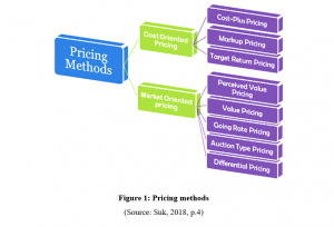
Price of products required to be reasonable and thus it is necessary to maintain the price products considering the market and operational costs of the company. As per the view of Agyei-Mensah, B.K., 2016, p.4), it can be said that the pricing methods are also divided into two parts wherein one part the price of products is determined based on costs of manufacturing and another is based on market condition. The costs plus pricing method is considered the simplest and widely used method where a certain profit margin is added over the total costs. The target return pricing is another cost-based pricing method where it utilizes the ROI in the calculation of pricing of products. On the other hand, the perceived value pricing is the pricing method based on the market demand and companies increase the price of the product and gain higher profit if there is a high demand for the products. As per the view of Suk (2018, p.4), Value pricing method considers the quality of products itself and it needs to reduce the cost price in order to serve a large number of audiences. It is also necessary to consider the price of opponent companies before setting the price of products and this method is known as going rate pricing.
a. Pricing method beneficial for the car market
Based on the discussion of different pricing methods it can be said that the value pricing method can be beneficial for the company as it considers the demands of the products. Further, it also can be said that as the demands of the product increases a car manufacturing company can enhance quality and safety. As per the view of Li and Trutnevyte (2017, p.90), based on the proper understanding of demands and supplies of the cars a company is easily able to grow the performance.
b. Required additional required for setting strategy
It can be said that the demand of the products depends on the customer’s choices, so it is essential to have sufficient knowledge of market demands in order to use a market oriented strategy. As per the view of Liu (2018, p.12), it can be said that opponents’ pricing helps to set the initial price of products, so there is a need for information about the opponent company.
3.2. Calculation of Income Statement
a. Income Statement under absorption costing
| Income statement | ||
| Absorption costing method | ||
| Sales | 3680000 | |
| Costs of sales:- | ||
| Beginning inventory | 275000 | |
| Production costs fixed | 350000 | |
| Direct variable costs | 2550000 | |
| Closing inventory | -720000 | |
| 2455000 | ||
| Gross Profit | 1225000 | |
| Operational Expenses:- | ||
| Selling fixed expenses | 140000 | |
| Selling variable overhead | 200000 | |
| Administrative overhead | 80000 | |
| 420000 | ||
| Operating profit | 805000 | |
Table 4: Calculation of Income Statement under absorption costing
(Source: Created by learner)
Income statement based on the absorption costing for Angle PLC has been prepared in order to find out the operating profit. Based on the calculation process total costs of sales have been calculated considering direct expenses and the amount of total expense is £2455000. Hence, after adjusting the costs of sales from net sales the gross profit has resulted as £1225000. Apart from that, selling and administrative overheads under operating expenses also been calculated so, total operating expenses were £420000. Therefore, operating profit under absorption costing method is £805000 which has been calculated by deducting operating expenses from gross profit.
b. Income Statement under marginal costing
| Income statement | ||
| Marginal costing method | ||
| Sales | 3680000 | |
| Variable costs:- | ||
| Opening stocks | 275000 | |
| Direct costs | 2550000 | |
| Selling expenses | 200000 | |
| 3025000 | ||
| Less: Closing Stocks | 495000 | |
| 2530000 | ||
| Contribution Margin | 1150000 | |
| Fixed Costs:- | ||
| Production overhead | 350000 | |
| Selling overhead | 140000 | |
| Administrative overhead | 80000 | |
| 570000 | ||
| Operating Profit | 580000 | |
Table 4: Calculation of Income Statement under marginal costing
(Source: Created by learner)
This section of the study has been conducted to prepare an income statement based on the marginal costing method. Based on the calculation process total variable costs has been founded amounting £2530000 while total sales were £3680000. Therefore, based on the calculation process total contribution has been calculated as £1150000. Apart from that, the total fixed costs of the company were £570000 and it is required to deduct from contribution in order to measure the profit. Hence, based on the marginal costing method net operating profit has been founded amounting of £580000.
c. Reconciliation of differences
| Reconciliation statement | ||
| Absorption to Marginal costing | ||
| Operating profit of absorption costing | 805000 | |
| Less: Fixed inventory expenses | 225000 | |
| Operating profit of marginal costing | 580000 | |
Table 5: Calculation of Reconciliation of differences
(Source: Created by learner)
The rectification of the income statement has represented the conversion of operating profit from absorption costing to the operating profit of marginal costing. Based on the calculation it is noticeable that there is an adjustment required regarding the position of fixed expenditure in closing stock. Therefore, £225000 fixed inventory expenditure has been adjusted from the operating profit of absorption costing in order to derive the result of operating profit of marginal costing.
d. Discussion regarding the reasons of differences
The marginal costing technique is based on the nature of costs while on the other hand absorption costs are based on the departments of costs. This is the basic reason for the difference in profit between the two results as marginal costing considers the physical condition of expenses while absorption costing considers the financial factor of the expenses. As per the view of Ul-Hameed et al. (2019, p.315), it has been found that the closing stock can be maintained at a selling price as it recorded in absorption costing. On the other hand, the marginal costing maintains the closing stock at manufacturing costs and fixed expenses and profit margin are being ignored.
3.3. Rationales for preparing zero-based budgeting
The process of budget helps to maintain the performance of the company so it is necessary for the management to prepare the budget accurately. As per the view of Suryanto, Haseeb and Hartani (2018, p.316), it can be seen that the zero-based budgeting is an effective way to maintain accuracy in the business as it begins making assumptions from the zero. It is necessary to cross-check in the financial information and this budgeting method takes a deep glance in market condition as well as present internal condition. As per the view of Esfahbodi, Zhang, Watson and Zhang (2017, p.67), resource allocation in the business is necessary and management requires to focus on the necessity of resource allocation instead of looking at the past result. As per the view of Nor and Ishak (2019, p.486), it can be seen that due to fluctuation in the market demand and supply often fluctuate thus the zero-based budgeting technique begins from scratch and is effective in such a scenario.
a. Explanation regarding feasibility for the company
Based on the rationale of zero-based budgeting it can be said that car manufacturing companies are required to maintain such a budget while planning for preparing a prototype. As per the view of Su (2018, p.14), present market demand and possible costs can be determined accurately with this type of budget planning. Apart from that, it is necessary for a car manufacturing company to reduce its costs and the zero-based budget planning is constructed from the zero so expenses can be monitored efficiently.
3.4. Market feasibility and possible selling price
a. Market feasibility of the product
Technology has enhanced its step forward at a rapid speed in this 21st century and it can be seen that the necessity of advanced technology will change the future of business. As per the view of Pillai et al. (2017, 86), it already can be seen that the internet of things and smart devices are able to enhance the quality of human life. Hence, it can be said that the video screen products can be a good way to generate revenue with low expenses. Clearly, it can be seen that the manufacturing of cars requires a high variable and fixed expenses however, the smart screen technology requires less effort investment. As per the view of Fang and Zhang (2018, p.65), it can be seen that the smart screen is already able to acquire a high demand thus, based on the observation of such companies detailed market information can be collected. Moreover, it can be seen that the market of the smart screen is compact with rival companies and competitions, so it can be assumed that there exists a high demand for the product. As per the view of Kim and Kim (2016, p.17), based on the controlling costs of manufacturing products it can be assumed that the company will be able to acquire the market of smart screen technology.
b. Determination of the Selling price of the product
| Costs:- | |
| Direct materials | 500000 |
| Direct labor | 250000 |
| Variable overhead | 125000 |
| 875000 | |
| Add: Depreciation | 100000 |
| Add: Corporate Exp | 300000 |
| 1275000 | |
| Add: Profit | 318750 |
| Total sales | 956250 |
| Selling Price | 38.25 |
Table 6: Calculation of selling price
(Source: Created by learner)
4. Conclusion
Financial analysis is necessary for the development and expansion of the business organization and a knowledgeable financial advisor able to provide proper advice regarding market risks. Based on the analysis of investment strategy it can be concluded that a company needs to follow investment appraisal techniques in order to gain an idea about the possible benefits of the project. It can be said that the calculation of costs of capital while trying to acquire funds for investment in a new sector helps in calculating investment appraisal techniques. Based on the outcome of NPV and IRR a company will be able to make proper decisions regarding the investment program. Apart from that, it also can be said that proper internal management is necessary for the reduction of costs as well as setting price considering market demands.
References
Agyei-Mensah, B.K., 2016. Internal control information disclosure and corporate governance: evidence from an emerging market. Corporate Governance: The international journal of business in society.
Batra, R. and Verma, S., 2018. Non-financial criteria in project appraisal methodologies: empirical evidence from Indian companies. International Journal of Accounting and Finance, 8(1), pp.80-102..
Bawaneh, S.S., 2018. MANAGEMENT ACCOUNTING PRACTICES: A CASE OF JORDANIAN MANUFACTURING COMPANIES. Asia-Pacific Management Accounting Journal, 13(3), pp.25-53.
Bolton, R., Foxon, T.J. and Hall, S., 2016. Energy transitions and uncertainty: Creating low carbon investment opportunities in the UK electricity sector. Environment and Planning C: Government and Policy, 34(8), pp.1387-1403.
Chang, A., 2017. Disclosure standards of large New Zealand companies: a content analysis study of compliance with the FMA’s corporate governance guidelines.
Esfahbodi, A., Zhang, Y., Watson, G. and Zhang, T., 2017. Governance pressures and performance outcomes of sustainable supply chain management–An empirical analysis of UK manufacturing industry. Journal of cleaner production, 155, pp.66-78.
Fang, C. and Zhang, J., 2018. Performance of green supply chain management: A systematic review and meta analysis. Journal of Cleaner Production, 183, pp.1064-1081.
Grant, R.M., 2016. Contemporary strategy analysis: Text and cases edition. John Wiley & Sons.
Kang, Y.Q., Xie, B.C., Wang, J. and Wang, Y.N., 2018. Environmental assessment and investment strategy for China’s manufacturing industry: A non-radial DEA based analysis. Journal of Cleaner Production, 175, pp.501-511.
Kim, C. and Kim, J., 2016. EMPIRICAL ANALYSIS FOR SUCCESS FACTORS IN UBIQUITOUS SUPPLY CHAIN MANAGEMENT IN THE CASE OF UK COMPANIES. Issues in Information Systems, 17(1).
Kim, J.R., 2019. A Comparison of Equity Valuation Models: Empirical Evidence from a Sample of UK Companies. European Journal of Multidisciplinary Studies, 4(2), pp.105-120.
Kobo, K.L. and Ngwakwe, C.C., 2017. Relating corporate social investment with financial performance. Investment Management and Financial Innovations, 14(2-2), pp.367-375.
Li, F.G. and Trutnevyte, E., 2017. Investment appraisal of cost-optimal and near-optimal pathways for the UK electricity sector transition to 2050. Applied energy, 189, pp.89-109.
Liu, M.L., 2018. Where does multinational investment go with territorial taxation? Evidence from the UK. International Monetary Fund.
Lluch, A., 2019. US Companies in Argentina: Trade and Investment Patterns (1890–1930). Journal of Evolutionary Studies in Business, 4(1), pp.70-108.
Maffini, G., Xing, J. and Devereux, M.P., 2019. The impact of investment incentives: evidence from UK corporation tax returns. American Economic Journal: Economic Policy, 11(3), pp.361-89.
Nor, M.N.M. and Ishak, S., 2019. An analysis of internal audit investment among top Malaysian listed companies. KnE Social Sciences, pp.485-497.
Pillai, K.V., Slutsky, P., Wolf, K., Duthler, G. and Stever, I., 2017. Companies’ Accountability in Sustainability: A Comparative Analysis of SDGs in Five Countries. In Sustainable development goals in the Asian context (pp. 85-106). Springer, Singapore.
Sciarelli, M., Landi, C.G., Turriziani, L. and Tani, M., 2019. Corporate Social Commitment from Investors’ Perspective: Evidences from Italian and UK Asset Management Companies. International Journal of Business and Social Science, 10(3).
Su, S., 2018, June. An Investigation of Foreign Exchange Risk Management in Chinese Multinational Companies Compared with US and UK MNEs. In 2018 2nd International Conference on Management, Education and Social Science (ICMESS 2018). Atlantis Press.
Suk, S., 2018. An Estimate of Internal Carbon Pricing of Korean Companies under the Emission Trading scheme. J. Clean. Prod.
Suryanto, T., Haseeb, M. and Hartani, N.H., 2018. The correlates of developing green supply chain management practices: Firms level analysis in Malaysia. International Journal of Supply Chain Management, 7(5), p.316.
Susu, S. and Birsan, M., 2019. Dynamics Of Profitability In Romanian Pharmaceutical Companies Under The Impact Of Changes In The Contemporary Business Environment. The USV Annals of Economics and Public Administration, 19(1 (29)), pp.122-134.
Ul-Hameed, W., Mohammad, H., Shahar, H., Aljumah, A. and Azizan, S., 2019. The effect of integration between audit and leadership on supply chain performance: Evidence from UK based supply chain companies. Uncertain Supply Chain Management, 7(2), pp.311-328.
Appendices
Annexure 1
| Calculation of Cost of debt | |
| [Bond Yield Approximation Method] | |
| Kd = | C + {(F-P) / n} |
| (F+P) / 2 | |
| Where, | |
| Kd = | Cost of Debt capital |
| C = | Payments of coupon = 10 |
| F = | Face value = 100 |
| P = | Selling Price = 105 |
| n = | Maturity period = 5 |
| Therefore, | |
| Kd = | 10 + {(100-105) / 5} |
| (100+105) / 2 | |
| Kd = | 9.0 |
| 102.5 | |
| Kd = | 8.78% |
| Calculation of Cost of preference share capital | |
| [Irredeemable] | |
| Kp = | D0 |
| P0 | |
| Where, | |
| Kp = | Cost of Preference share capital |
| D0 = | Industry average preferred dividend = 10 |
| P0 = | Current market price = 98 |
| Therefore, | |
| Kp = | 10 |
| 98 | |
| Kp = | 10.20% |
| Calculation of Cost of Equity | |
| [Dividend Discount Model] | |
| Ke = | {D1 / (P0 – F)} + g |
| Where, | |
| Ke = | Cost of equity share capital |
| D0 = | Dividend per share = 1.2 |
| D1 = | Expected Dividend per share = 1.31 |
| P0 = | Market price per share = 34.80 |
| F = | Floatation Costs = 10*20% = 2 |
| g = | Growth rate = 9% = 0.09 |
| Therefore, | |
| Ke = | {1.31 / (34.80 – 2 )} + 0.09 |
| Ke = | 13.0% |
| Calculation of Cost of Equity | |
| [Capital Asset Pricing Model] | |
| Ke = | RF + bi (RM – RF) |
| Where, | |
| Ke = | Cost of equity share capital |
| RF = | Risk Free rate of return = 0.03 |
| bi = | Beta of Stock = 1.5 |
| RM = | Market rate of return = 0.10 |
| Ke = | 0.03 + 1.5 (0.10 – 0.03) |
| Ke = | 13.50% |
Table 1: Calculation of costs of capital
(Source: Created by learner)
Annexure 2
| Calculation of optimum cost of capital | |||
| [Weighted Average Cost of Capital] [DDM] | |||
| Capital structure policy | Cost of capital | ||
| Ke | 0.4000 | 12.99% | 5.20% |
| Kp | 0.1000 | 10.20% | 1.02% |
| Kd | 0.5000 | 8.78% | 4.39% |
| 1 | WACC = | 10.61% | |
| Calculation of optimum cost of capital | |||
| [Weighted Average Cost of Capital] [CAPM] | |||
| Capital structure policy | Cost of capital | ||
| Ke | 0.4000 | 13.50% | 5.40% |
| Kp | 0.1000 | 10.20% | 1.02% |
| Kd | 0.5000 | 8.78% | 4.39% |
| 1 | WACC = | 10.81% | |
Table 2: Calculation of optimum cost of capital (WACC)
(Source: Created by learner)
Annexure 3
| 1 | 2 | 3 | 4 | 5 | |
| 2020 | 2021 | 2022 | 2023 | 2024 | |
| Expected unit | 8,000 | 8,000 | 10,000 | 11,000 | 12,000 |
| Unit Price | 30,000 | 30,000 | 30,000 | 31,000 | 31,000 |
| Sales Revenue | 240,000,000 | 240,000,000 | 300,000,000 | 341,000,000 | 372,000,000 |
| Production Costs PU | 15,000 | 15,750 | 16,538 | 17,364 | 18,233 |
| Total Production costs | 120,000,000 | 126,000,000 | 165,375,000 | 191,008,125 | 218,791,125 |
| Contribution | 120,000,000 | 114,000,000 | 134,625,000 | 149,991,875 | 153,208,875 |
| Fixed Cost | 20,000,000 | 20,000,000 | 15,000,000 | 10,000,000 | 10,000,000 |
| Promotion and R&D | 5,000,000 | 5,000,000 | 5,000,000 | 5,000,000 | 5,000,000 |
| Depreciation | 27,000,000 | 27,000,000 | 27,000,000 | 27,000,000 | 27,000,000 |
| Operating Profit(PBIT) | 68,000,000 | 62,000,000 | 87,625,000 | 107,991,875 | 111,208,875 |
| Corporation Tax | 20,400,000 | 18,600,000 | 26,287,500 | 32,397,563 | 33,362,663 |
| Profit after Tax | 47,600,000 | 43,400,000 | 61,337,500 | 75,594,313 | 77,846,213 |
| Initial Investment | – 150,000,000 | ||||
| Net CF | 74,600,000 | 70,400,000 | 88,337,500 | 102,594,313 | 104,846,213 |
| a) | |||||
| PV @10.61% | 67,444,173 | 57,541,857 | 65,277,262 | 68,540,255 | 63,325,815 |
| NPV @10.61% | 322,129,362 | ||||
| b) | |||||
| PV @10.81% | 67,322,444 | 57,334,331 | 64,924,444 | 68,046,762 | 62,756,393 |
| NPV @10.81% | 320,384,374 | ||||
| IRR = | ra + [{Na * (rb – ra)} / (Na – Nb)] | ||||
| Here, | |||||
| ra = lower discount rate = | 10.61 | ||||
| rb = higher discount rate = | 10.81 | ||||
| Na = NPV at lower discount rate = | 322,129,361.59 | ||||
| Nb = NPV at higher discount rate = | 320,384,373.93 | ||||
| Therefore, | |||||
| IRR = | 48% | ||||
Table 3: Calculation of total value addition (NPV) and break even rate (IRR)
(Source: Created by learner)
Annexure 4
Annexure 5
| Income statement | ||
| Absorption costing method | ||
| Sales | 3680000 | |
| Costs of sales:- | ||
| Beginning inventory | 275000 | |
| Production costs fixed | 350000 | |
| Direct variable costs | 2550000 | |
| Closing inventory | -720000 | |
| 2455000 | ||
| Gross Profit | 1225000 | |
| Operational Expenses:- | ||
| Selling fixed expenses | 140000 | |
| Selling variable overhead | 200000 | |
| Administrative overhead | 80000 | |
| 420000 | ||
| Operating profit | 805000 | |
Table 4: Calculation of Income Statement under absorption costing
(Source: Created by learner)
Annexure 6
| Income statement | ||
| Marginal costing method | ||
| Sales | 3680000 | |
| Variable costs:- | ||
| Opening stocks | 275000 | |
| Direct costs | 2550000 | |
| Selling expenses | 200000 | |
| 3025000 | ||
| Less: Closing Stocks | 495000 | |
| 2530000 | ||
| Contribution Margin | 1150000 | |
| Fixed Costs:- | ||
| Production overhead | 350000 | |
| Selling overhead | 140000 | |
| Administrative overhead | 80000 | |
| 570000 | ||
| Operating Profit | 580000 | |
Table 4: Calculation of Income Statement under marginal costing
(Source: Created by learner)
Annexure 7
| Reconciliation statement | ||
| Absorption to Marginal costing | ||
| Operating profit of absorption costing | 805000 | |
| Less: Fixed inventory expenses | 225000 | |
| Operating profit of marginal costing | 580000 | |
Table 5: Calculation of Reconciliation of differences
(Source: Created by learner)
Annexure 8
| Costs:- | |
| Direct materials | 500000 |
| Direct labor | 250000 |
| Variable overhead | 125000 |
| 875000 | |
| Add: Depreciation | 100000 |
| Add: Corporate Exp | 300000 |
| 1275000 | |
| Add: Profit | 318750 |
| Total sales | 956250 |
| Selling Price | 38.25 |
Table 6: Calculation of selling price
(Source: Created by learner)
________________________________________________________________________________
Know more about UniqueSubmission’s other writing services:
