
ASSIGNMENT FOR RESEARCH METHODS AND DATA ANALYSIS
Exercise 1a
| Case Processing Summary | ||||||
| Cases | ||||||
| Valid | Missing | Total | ||||
| N | Percent | N | Percent | N | Percent | |
| cholesterol values in mmol/L | 44 | 100.0% | 0 | 0.0% | 44 | 100.0% |
As all the variables have same value which indicates the null missing value in the statistics in the field of normality of the following distribution of cholesterol values.
| Descriptives | ||||
| Statistic | Std. Error | |||
| cholesterol values in mmol/L | Mean | 5.9932 | .23706 | |
| 95% Confidence Interval for Mean | Lower Bound | 5.5151 | ||
| Upper Bound | 6.4713 | |||
| 5% Trimmed Mean | 6.0162 | |||
| Median | 5.7500 | |||
| Variance | 2.473 | |||
| Std. Deviation | 1.57250 | |||
| Minimum | 3.00 | |||
| Maximum | 8.50 | |||
| Range | 5.50 | |||
| Interquartile Range | 2.50 | |||
| Skewness | -.184 | .357 | ||
| Kurtosis | -.980 | .702 | ||

From the descriptive values, it has been analysed that the mean of the cholesterol value is 5.99 with standard error of 0.24 and 5% trimmed mean is reflected as 6.01. The median, variance and standard deviation for cholesterol values are 5.75, 2.473 and 1.572 respectively.
On the other hand, the values of skewness and kurtosis is need to be approximately zero for constructing the table using normal distribution. The kurtosis is -0.980 with standard error of 0.702 which reflects the pattern of normal distribution.
| Tests of Normality | ||||||
| Kolmogorov-Smirnova | Shapiro-Wilk | |||||
| Statistic | df | Sig. | Statistic | df | Sig. | |
| cholesterol values in mmol/L | .105 | 44 | .200* | .959 | 44 | .121 |
| *. This is a lower bound of the true significance. | ||||||
| a. Lilliefors Significance Correction
|
||||||
Shapiro-Wilk test highlights if the random sample is obtained from normal distribution and it is a test of normality (Hanusz, et al., 2016). Kolmogorov–Smirnov test (KS test) helps to determine if the datasets vary significantly or not (Hassani & Silva, 2015). The normal distribution test or test of normality has been conducted through following Shapiro-Wilk test and KS test.
The value of statistical significant differs with that of normal distribution. The null-hypothesis of the normal distribution is rejected if the value is less than 0.05 which has also reflected the non-normal distribution. The significant value of cholesterol is 0.20 which indicates that it is distributed normally with having null-hypothesis.
From the Shapiro-Wilk test, it has been found that the significant value for cholesterol is 0.121 which is greater than 0.05. So, the cholesterol values are stated to be normally distributed. Shapiro-Wilk test is also considered as very useful in the cases where the number of observations is very much less in relation with the same value.
Shapiro-Wilk test is also considered as very useful in the cases where the number of observations is very much less in relation with the same value.
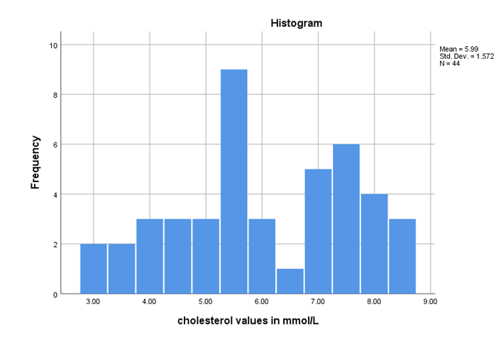
From the histogram, it has been stated that the range of the value lies in between 3 to 9 which reflects the continuous measurement of variables. The results have shown that the standard deviation is 1.57 for the sample size 44 and the histogram also reflects the standard median of 5.75.
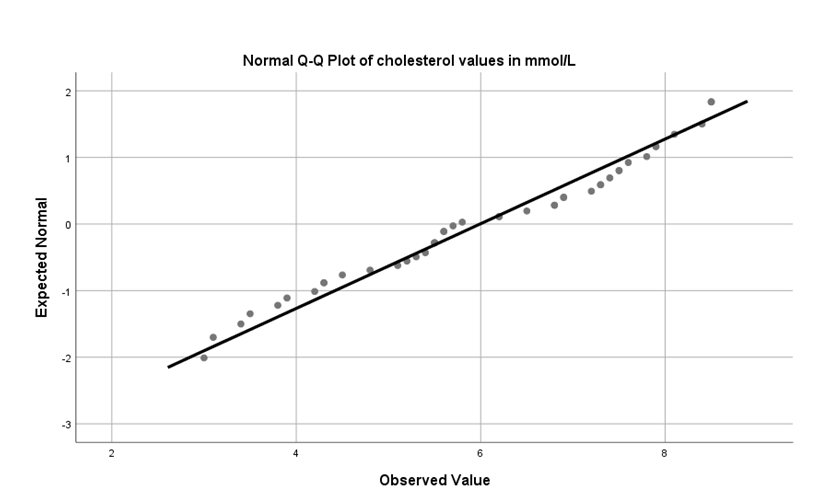
The normal Q-Q plot of cholesterol values reflects that the observed values of the limit will be hugging with the line which indicates the normal distribution of the variables. By checking each section of the variable category, it has been stated that the cholesterol values are approximated normally distributed.
The difference in outliers is demonstrated through the detrended normal Q-Q plot which reflects that the observed values have differed with that of the standard one. The pattern of Q-Q curve helps to showcase the approximated normal distribution of identified cholesterol values.
From the figure of Boxplot, it has been identified that the line across the summary plot indicates its median of 5.75 and outliers belong to the range of 3 to 8.5.
Exercise 1b
| Statistics | ||
| cholesterol values in mmol/L | ||
| N | Valid | 44 |
| Missing | 0 | |
| Mean | 5.9932 | |
| Median | 5.7500 | |
| Mode | 5.50 | |
| Std. Deviation | 1.57250 | |
| Variance | 2.473 | |
| Range | 5.50 | |
| Minimum | 3.00 | |
| Maximum | 8.50 | |
From the statistics, it has been analysed that the null hypothesis is not included in the cholesterol values and the mean, mode and median of the dataset are identified as 5.99, 5.50 and 5.75 respectively.
Having the variance of the sample as 2.47, the maximum and minimum sample is also identified as 8.5 and 3 respectively. Moreover, 95% of the distributed sample of cholesterol are included under confidence interval which is also reflected from the below figure.
From the histogram, it has been stated that the range of the value lies in between 3 to 9 which reflects the continuous measurement of variables. The results have shown that the standard deviation is 1.57 for the sample size 44 and the histogram also reflects the standard median of 5.75.
The original or true value must lie in between the upper and lower limit of 95% confidence interval which reflects the normal distribution.
| Paired Samples Statistics | |||||
| Mean | N | Std. Deviation | Std. Error Mean | ||
| Pair 1 | aerobic capacity for group 1 | 46.3462 | 13 | 8.13794 | 2.25706 |
| aerobic capacity for group 2 | 34.3692 | 13 | 6.86590 | 1.90426 | |
| Pair 2 | systolic blood pressure for group 1 | 122.7692 | 13 | 3.72276 | 1.03251 |
| systolic blood pressure for group 2 | 136.5385 | 13 | 5.79677 | 1.60774 | |
| Pair 3 | body fat for group 1 | 21.5000 | 13 | 5.13566 | 1.42438 |
| body fat for group 2 | 32.1154 | 13 | 3.68077 | 1.02086 | |
For developing the hypothesis, the group of participants is distributed on the basis of three pairs which are aerobic capacity, systolic blood pressure and body fat. For the constant sample size of 13, the mean and standard deviation for thehealthy weight group is 46.34 and 8.13 respectively. The mean and standard deviation forthe overweight group for SBP are 136.53 and 5.79 respectively.
| Paired Samples Correlations | ||||
| N | Correlation | Sig. | ||
| Pair 1 | aerobic capacity for group 1 & aerobic capacity for group 2 | 13 | .087 | .778 |
| Pair 2 | systolic blood pressure for group 1 & systolic blood pressure for group 2 | 13 | .134 | .663 |
| Pair 3 | body fat for group 1 & body fat for group 2 | 13 | -.179 | .559 |
From the paired samples correlations, it has been identified that the significant values for aerobic capacity for group 1 & aerobic capacity for group 2 along with systolic blood pressure for group 1 & systolic blood pressure for group 2 are 0.778 and 0.663 respectively. On the other hand, the correlation and significant value of body fat for group 1 & body fat for group 2 are -0.179 and 0.559 respectively.
| Paired Samples Test | |||||||||
| Paired Differences | t | df | Sig. (2-tailed) | ||||||
| Mean | Std. Deviation | Std. Error Mean | 95% Confidence Interval of the Difference | ||||||
| Lower | Upper | ||||||||
| Pair 1 | aerobic capacity for group 1 – aerobic capacity for group 2 | 11.97692 | 10.18194 | 2.82396 | 5.82404 | 18.12981 | 4.241 | 12 | .001 |
| Pair 2 | systolic blood pressure for group 1 – systolic blood pressure for group 2 | -13.76923 | 6.45696 | 1.79084 | -17.67113 | -9.86733 | -7.689 | 12 | .000 |
| Pair 3 | body fat for group 1 – body fat for group 2 | -10.61538 | 6.83177 | 1.89479 | -14.74378 | -6.48699 | -5.602 | 12 | .000 |
Paired sample test are normally carried out to evaluate if the mean difference between two data sets is zero or not (Skyttberg, et al., 2018).From the paired sample test, it has been identified that the difference between two datasets have been equivalent from the value of t in T-testing.
The standard error mean of three dataset is identified as 2.82, 1.79 and 1.894 respectively. The original or true value must lie in between the upper and lower limit of 95% confidence interval which reflects the normal distribution.
| Paired Samples Statistics | |||||
| Mean | N | Std. Deviation | Std. Error Mean | ||
| Pair 1 | aerobic capacity for group 2 | 34.3692 | 13 | 6.86590 | 1.90426 |
| group 2 retest for AC | 36.4077 | 13 | 5.14546 | 1.42709 | |
For the group of overweight, it has been identified that the standard deviation has been changed from 6.86 to 5.14 which demonstrates the slight change after training.
| Paired Samples Correlations | ||||
| N | Correlation | Sig. | ||
| Pair 1 | aerobic capacity for group 2 & group 2 retest for AC | 13 | .912 | .000 |
For the sample size of 13, the correlation of the aerobic capacity for group 2 is demonstrated as 0.912.
| Paired Samples Test | |||||||||
| Paired Differences | t | df | Sig. (2-tailed) | ||||||
| Mean | Std. Deviation | Std. Error Mean | 95% Confidence Interval of the Difference | ||||||
| Lower | Upper | ||||||||
| Pair 1 | aerobic capacity for group 2 – group 2 retest for AC | -2.03846 | 3.02587 | .83923 | -3.86698 | -.20995 | -2.429 | 12 | .032 |
The original or true value must lie in between – 3.86 to -0.209 of 95% confidence interval which reflects the normal distribution. The mean of the group is also identified as 2.03 with standard deviation of 3.025.
| Correlations | ||||
| systolic bp | diastolic bp | age | ||
| systolic bp | Pearson Correlation | 1 | .725** | .223 |
| Sig. (2-tailed) | .000 | .124 | ||
| N | 49 | 49 | 49 | |
| diastolic bp | Pearson Correlation | .725** | 1 | .365** |
| Sig. (2-tailed) | .000 | .010 | ||
| N | 49 | 49 | 49 | |
| age | Pearson Correlation | .223 | .365** | 1 |
| Sig. (2-tailed) | .124 | .010 | ||
| N | 49 | 49 | 49 | |
| **. Correlation is significant at the 0.01 level (2-tailed). | ||||
Based on the Bivariate relationship table above, it is seen that diastolic blood pressure and systolic blood pressure has the highest correlation with 0.725, followed by the diastolic blood pressure and age with 0.365 and systolic blood pressure and age with 0.223.
| Descriptives | |||||||||
| N | Mean | Std. Deviation | Std. Error | 95% Confidence Interval for Mean | Minimum | Maximum | |||
| Lower Bound | Upper Bound | ||||||||
| Atkins Diet | 25 | 2 | 54.50 | 36.062 | 25.500 | -269.51 | 378.51 | 29 | 80 |
| 32 | 1 | 37.00 | . | . | . | . | 37 | 37 | |
| 36 | 1 | 40.00 | . | . | . | . | 40 | 40 | |
| 39 | 1 | 48.00 | . | . | . | . | 48 | 48 | |
| 40 | 1 | 65.00 | . | . | . | . | 65 | 65 | |
| 41 | 1 | 66.00 | . | . | . | . | 66 | 66 | |
| 49 | 2 | 57.00 | 4.243 | 3.000 | 18.88 | 95.12 | 54 | 60 | |
| 50 | 1 | 58.00 | . | . | . | . | 58 | 58 | |
| 51 | 1 | 63.00 | . | . | . | . | 63 | 63 | |
| 52 | 1 | 57.00 | . | . | . | . | 57 | 57 | |
| 58 | 2 | 55.00 | 7.071 | 5.000 | -8.53 | 118.53 | 50 | 60 | |
| 60 | 1 | 70.00 | . | . | . | . | 70 | 70 | |
| 61 | 1 | 70.00 | . | . | . | . | 70 | 70 | |
| 72 | 1 | 73.00 | . | . | . | . | 73 | 73 | |
| Total | 17 | 57.65 | 13.527 | 3.281 | 50.69 | 64.60 | 29 | 80 | |
| 5:2 Diet | 25 | 2 | 39.00 | 29.698 | 21.000 | -227.83 | 305.83 | 18 | 60 |
| 32 | 1 | 25.00 | . | . | . | . | 25 | 25 | |
| 36 | 1 | 28.00 | . | . | . | . | 28 | 28 | |
| 39 | 1 | 44.00 | . | . | . | . | 44 | 44 | |
| 40 | 1 | 45.00 | . | . | . | . | 45 | 45 | |
| 41 | 1 | 59.00 | . | . | . | . | 59 | 59 | |
| 49 | 2 | 46.00 | 5.657 | 4.000 | -4.82 | 96.82 | 42 | 50 | |
| 50 | 1 | 54.00 | . | . | . | . | 54 | 54 | |
| 51 | 1 | 68.00 | . | . | . | . | 68 | 68 | |
| 52 | 1 | 47.00 | . | . | . | . | 47 | 47 | |
| 58 | 2 | 55.50 | .707 | .500 | 49.15 | 61.85 | 55 | 56 | |
| 60 | 1 | 63.00 | . | . | . | . | 63 | 63 | |
| 61 | 1 | 55.00 | . | . | . | . | 55 | 55 | |
| 72 | 1 | 75.00 | . | . | . | . | 75 | 75 | |
| Total | 17 | 49.65 | 15.137 | 3.671 | 41.86 | 57.43 | 18 | 75 | |
| ANOVA | ||||||
| Sum of Squares | df | Mean Square | F | Sig. | ||
| Atkins Diet | Between Groups | 1559.382 | 13 | 119.952 | .263 | .963 |
| Within Groups | 1368.500 | 3 | 456.167 | |||
| Total | 2927.882 | 16 | ||||
| 5:2 Diet | Between Groups | 2751.382 | 13 | 211.645 | .694 | .724 |
| Within Groups | 914.500 | 3 | 304.833 | |||
| Total | 3665.882 | 16 | ||||
Null hypothesis: There is no difference in the preference of a particular diet.
Alternate hypothesis: There is a significant difference in the preference of a particular diet.
One–way Anova test helps to find out if there is a variance between the means of independent variables (Kim, 2017). Based on one–way Anova test result, the significance value for both Atkins diet and 5:2 diet with relation to low-calorie diet is higher than the significance value of 0.05.
Therefore, null hypothesis is accepted. Since the significance value as suggested by Anova test is above 0.05 for both the variables, therefore there is no need for post hoc tests.
| Descriptives | ||||||||
| systolic BP | ||||||||
| N | Mean | Std. Deviation | Std. Error | 95% Confidence Interval for Mean | Minimum | Maximum | ||
| Lower Bound | Upper Bound | |||||||
| 6 weeks | 10 | 187.4000 | 12.94604 | 4.09390 | 178.1390 | 196.6610 | 170.00 | 210.00 |
| 12 weeks | 7 | 179.0000 | 14.23610 | 5.38074 | 165.8338 | 192.1662 | 159.00 | 200.00 |
| 24 weeks | 6 | 163.5000 | 4.96991 | 2.02896 | 158.2844 | 168.7156 | 155.00 | 169.00 |
| Total | 23 | 178.6087 | 15.06271 | 3.14079 | 172.0951 | 185.1223 | 155.00 | 210.00 |
| ANOVA | |||||
| systolic BP | |||||
| Sum of Squares | df | Mean Square | F | Sig. | |
| Between Groups | 2143.578 | 2 | 1071.789 | 7.527 | .004 |
| Within Groups | 2847.900 | 20 | 142.395 | ||
| Total | 4991.478 | 22 | |||
Post Hoc Tests
| Multiple Comparisons | ||||||
| Dependent Variable: systolic BP | ||||||
| Tukey HSD | ||||||
| (I) Group | (J) Group | Mean Difference (I-J) | Std. Error | Sig. | 95% Confidence Interval | |
| Lower Bound | Upper Bound | |||||
| 6 weeks | 12 weeks | 8.40000 | 5.88062 | .346 | -6.4779 | 23.2779 |
| 24 weeks | 23.90000* | 6.16214 | .003 | 8.3099 | 39.4901 | |
| 12 weeks | 6 weeks | -8.40000 | 5.88062 | .346 | -23.2779 | 6.4779 |
| 24 weeks | 15.50000 | 6.63887 | .074 | -1.2962 | 32.2962 | |
| 24 weeks | 6 weeks | -23.90000* | 6.16214 | .003 | -39.4901 | -8.3099 |
| 12 weeks | -15.50000 | 6.63887 | .074 | -32.2962 | 1.2962 | |
| *. The mean difference is significant at the 0.05 level. | ||||||
From the results of the Anova test, it can be said that there is a statistical significant difference between the levels of the independent variables i.e. difference is observed in systolic blood pressure due to the exercise lasting for 24 weeks, 12 weeks and 6 weeks.
The significant difference in the Anova test can be found out through Post hoc where except the significance value of 24 weeks and 6 weeks, all other values have more than 0.05 significance. Therefore all the values except the significance value of 24 weeks and 6 weeks have a non-statistically significant difference.
| Between-Subjects Factors | |||
| Value Label | N | ||
| Main Sport participated in | 1 | Runner | 8 |
| 2 | Rower | 8 | |
| Multivariate Testsa | ||||||
| Effect | Value | F | Hypothesis df | Error df | Sig. | |
| heartrate | Pillai’s Trace | .971 | 37.635b | 7.000 | 8.000 | .000 |
| Wilks’ Lambda | .029 | 37.635b | 7.000 | 8.000 | .000 | |
| Hotelling’s Trace | 32.931 | 37.635b | 7.000 | 8.000 | .000 | |
| Roy’s Largest Root | 32.931 | 37.635b | 7.000 | 8.000 | .000 | |
| heartrate * sport | Pillai’s Trace | .641 | 2.038b | 7.000 | 8.000 | .170 |
| Wilks’ Lambda | .359 | 2.038b | 7.000 | 8.000 | .170 | |
| Hotelling’s Trace | 1.783 | 2.038b | 7.000 | 8.000 | .170 | |
| Roy’s Largest Root | 1.783 | 2.038b | 7.000 | 8.000 | .170 | |
| a. Design: Intercept + sport
Within Subjects Design: heartrate |
||||||
| b. Exact statistic | ||||||
| Mauchly’s Test of Sphericitya | |||||||
| Measure: MEASURE_1 | |||||||
| Within Subjects Effect | Mauchly’s W | Approx. Chi-Square | df | Sig. | Epsilonb | ||
| Greenhouse-Geisser | Huynh-Feldt | Lower-bound | |||||
| heartrate | .001 | 81.311 | 27 | .000 | .411 | .565 | .143 |
| Tests the null hypothesis that the error covariance matrix of the orthonormalized transformed dependent variables is proportional to an identity matrix. | |||||||
| a. Design: Intercept + sport
Within Subjects Design: heartrate |
|||||||
| b. May be used to adjust the degrees of freedom for the averaged tests of significance. Corrected tests are displayed in the Tests of Within-Subjects Effects table. | |||||||
| Tests of Within-Subjects Effects | ||||||
| Measure: MEASURE_1 | ||||||
| Source | Type III Sum of Squares | df | Mean Square | F | Sig. | |
| heartrate | Sphericity Assumed | 15918.094 | 7 | 2274.013 | 87.152 | .000 |
| Greenhouse-Geisser | 15918.094 | 2.876 | 5535.544 | 87.152 | .000 | |
| Huynh-Feldt | 15918.094 | 3.956 | 4023.623 | 87.152 | .000 | |
| Lower-bound | 15918.094 | 1.000 | 15918.094 | 87.152 | .000 | |
| heartrate * sport | Sphericity Assumed | 190.844 | 7 | 27.263 | 1.045 | .405 |
| Greenhouse-Geisser | 190.844 | 2.876 | 66.366 | 1.045 | .381 | |
| Huynh-Feldt | 190.844 | 3.956 | 48.240 | 1.045 | .392 | |
| Lower-bound | 190.844 | 1.000 | 190.844 | 1.045 | .324 | |
| Error(heartrate) | Sphericity Assumed | 2557.063 | 98 | 26.092 | ||
| Greenhouse-Geisser | 2557.063 | 40.259 | 63.516 | |||
| Huynh-Feldt | 2557.063 | 55.386 | 46.168 | |||
| Lower-bound | 2557.063 | 14.000 | 182.647 | |||
| Tests of Within-Subjects Contrasts | ||||||
| Measure: MEASURE_1 | ||||||
| Source | heartrate | Type III Sum of Squares | df | Mean Square | F | Sig. |
| heartrate | Linear | 3043.006 | 1 | 3043.006 | 42.968 | .000 |
| Quadratic | 30.006 | 1 | 30.006 | 2.137 | .166 | |
| Cubic | 6436.031 | 1 | 6436.031 | 148.967 | .000 | |
| Order 4 | .274 | 1 | .274 | .017 | .899 | |
| Order 5 | 2849.144 | 1 | 2849.144 | 133.314 | .000 | |
| Order 6 | 16.751 | 1 | 16.751 | 4.524 | .052 | |
| Order 7 | 3542.881 | 1 | 3542.881 | 271.684 | .000 | |
| heartrate * sport | Linear | 17.357 | 1 | 17.357 | .245 | .628 |
| Quadratic | 44.024 | 1 | 44.024 | 3.135 | .098 | |
| Cubic | 62.546 | 1 | 62.546 | 1.448 | .249 | |
| Order 4 | 24.961 | 1 | 24.961 | 1.516 | .238 | |
| Order 5 | 6.322 | 1 | 6.322 | .296 | .595 | |
| Order 6 | 5.046 | 1 | 5.046 | 1.363 | .263 | |
| Order 7 | 30.587 | 1 | 30.587 | 2.346 | .148 | |
| Error(heartrate) | Linear | 991.494 | 14 | 70.821 | ||
| Quadratic | 196.613 | 14 | 14.044 | |||
| Cubic | 604.862 | 14 | 43.204 | |||
| Order 4 | 230.485 | 14 | 16.463 | |||
| Order 5 | 299.203 | 14 | 21.372 | |||
| Order 6 | 51.839 | 14 | 3.703 | |||
| Order 7 | 182.566 | 14 | 13.040 | |||
| Tests of Between-Subjects Effects | |||||
| Measure: MEASURE_1 | |||||
| Transformed Variable: Average | |||||
| Source | Type III Sum of Squares | df | Mean Square | F | Sig. |
| Intercept | 3292819.531 | 1 | 3292819.531 | 5790.345 | .000 |
| sport | 3549.031 | 1 | 3549.031 | 6.241 | .026 |
| Error | 7961.437 | 14 | 568.674 | ||
Based on the significant value provided in Tests of Within-Subjects Contrasts table, it is seen that for eight separate heart rate variables, the significance value is less than 0.05. But heartrate * sport source leads to the significance values of higher than 0.05. Test of between-subjects effects also showed that the significance value of sport is less than 0.05. From the above graph between heart rate and estimated marginal means, it is observed that the rowers showed higher heart rates in comparison to runners.
References
Hanusz, Z., Tarasinska, J. & Zielinski, W., 2016. Shapiro-Wilk test with known mean. REVSTAT-Statistical Journal, 14(1), pp. 89-100.
Hassani, H. & Silva, E., 2015. A Kolmogorov-Smirnov based test for comparing the predictive accuracy of two sets of forecasts. Econometrics, 3(3), pp. 590-609.
Kim, T., 2017. Understanding one-way ANOVA using conceptual figures. Korean journal of anesthesiology, 70(1), p. 22.
Skyttberg, N., Chen, R. & Koch, S., 2018. Man vs machine in emergency medicine–a study on the effects of manual and automatic vital sign documentation on data quality and perceived workload, using observational paired sample data and questionnaires. BMC, 18(1), p. 54.
