Statistics and Forecasting Assignment Sample

Introduction

Economic statistics encompass any mathematical information which summarises previous activity or projects upcoming behaviour of a single capital product, a series of instruments, or marketplaces in a large geographical area. It is helpful to divide such statistics into 3 groups initially. Forecasting is a strategy which utilises previous information as insight to create accurate predictions about the route of upcoming developments. Forecasting is used by organisations to effectively manage their resources or prepare for unexpected costs in the future. Statistics and forecasting is a combination that is utilised by several sectors like stock markets, GDP analysis, product purchases and many more for the development. In this project the developer will try to analyse the concept and prepare a high accuracy model with the help of SPSS software.

Methodology

This research applied primary analysis to achieve their project aim and the complete dataset which is collected is passed through the pre data processing for an accurate result. Developers conducted two analysis processes, one is for the first case study where university teacher’s salary related problems are covered and in the second case study company’s size and their cooperation related effectiveness is mentioned.

Topic 1

First case study is about the US universities faculty members’ salary, where 787 participants contributed their point of view and those responses are considered as a dataset. The empirical study was conducted for some issues like the interviewer wanted to know about the faculty members phD years, salary, gender and also their designation, etc.

Determining Causal Factors

Here Dependent variable is Salary

Here chosen Independent Variable is Female/Male, Position, University, State, and Publication

In the collected dataset few minor errors are present but those errors are identified and rectified while the dataset is passing through the pre-processing phase. Developers determine the required causal factors with the help of correlation analysis and means analysis. In causal factor analysis developers determine the mean, median, standard deviation, error difference and the correlation between independent and dependent variables. This total analysis part is performed in the SPSS software (Á. and Zilberman, 2021.). To analyse the first case study the developers operate two regression methods one is Durbin-Watson test and the other one is VIF. These two analyses help the developers to gain the impact of the gender, position, university, etc. on their salary structure. Several issues are present in the university related to the teacher’s salary and this project conducted by the developers to establish a model which helps the university to identify what type of issues are available and how much the independent variables affect the dependent variable.

Dataset for Case Study 1:

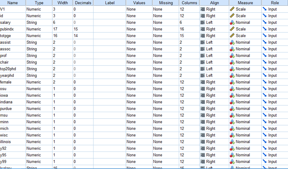Figure 1: Dataset

(Source: Case study file)

Topic 2

Second case study about the UK based company’s innovation activities and their effectiveness or impact. Developers in this project try to establish a relationship or determine the impact of the independent and dependent variables on the UK based companies.

Determining Causal Factors

The Dependent variable is Innovation

The Independent Variable is Size and Cooperation

In this second case study the developers collected the dataset via primary research method and for that they passed the data through a pre-processing step where some errors are recognised and eliminated from the dataset (Vasconcelos, et al. 2021.). Developers again determine the causal factors for the second case study where they analyse correlation analysis and means analysis. Here the developers determine the mean, median, standard deviation, error difference and the correlation between independent and dependent variables. In this particular case study helps the developers to understand the impact of any company’s size as well as their cooperation activities on their innovation system. For appropriate results the developers perform ANOVA as well as cluster analysis.

Analysis and Result

Topic 1

Causal Factors

Means

Means analysis is performed by the developers where they consider salary as a dependent variable and female, position, university and state as an independent variable (Medeiros, et al. 2021. ). After means analysis developers get mean, median, standard deviation, error difference, maximum, minimum and range. The developers determine each and every independent variable’s mean, median, standard deviation, range, etc with respect to dependent variables. The result shows in the tables below which is the processing of the given case study.


	Cases
	Included		Excluded		Total
	N	Percent	N	Percent	N	Percent
salary * prof	679	86.4%	107	13.6%	786	100.0%
salary * pubindx	679	86.4%	107	13.6%	786	100.0%
salary * female	664	84.5%	122	15.5%	786	100.0%
salary * osu	679	86.4%	107	13.6%	786	100.0%
salary * indiana	679	86.4%	107	13.6%	786	100.0%

*salary prof**
salary
prof	Mean	Std. Deviation	Std. Error of Mean	Minimum	Maximum	Range	Median
0	60574.77	14725.871	1122.837	18670	118962	100292	57721.00
1	93267.48	25672.520	1278.839	38200	191000	152800	89500.00
NA	74065.45	31046.216	3044.332	22254	223537	201283	66056.00
Total	82044.86	28168.631	1081.013	18670	223537	204867	78371.00

*salary female**
salary
female	Mean	Std. Deviation	Std. Error of Mean	Minimum	Maximum	Range	Median
0	83776.46	28210.024	1145.954	18670	223537	204867	80043.00
1	68319.62	22946.900	3013.076	36050	139660	103610	61464.00
Total	82426.31	28116.404	1091.128	18670	223537	204867	78550.00

*salary osu**
salary
osu	Mean	Std. Deviation	Std. Error of Mean	Minimum	Maximum	Range	Median
0	81798.40	28100.871	1151.057	18670	223537	204867	78290.00
1	83814.64	28761.133	3156.945	42648	181104	138456	78492.00
Total	82044.86	28168.631	1081.013	18670	223537	204867	78371.00

*salary indiana**
salary
indiana	Mean	Std. Deviation	Std. Error of Mean	Minimum	Maximum	Range	Median
0	82254.70	28139.148	1126.467	18670	223537	204867	78550.00
1	79664.15	28653.749	3863.671	36050	191000	154950	74107.00
Total	82044.86	28168.631	1081.013	18670	223537	204867	78371.00

Correlation

Correlation assessment is generally a statistical tool applied in exploration to determine the intensity of a logistic connection across two factors as well as calculate their associations. Specifically stated, correlation investigation or examination computes the quantity of changes in one variable like a result of a variation into some other variables (P. and Loeffler, 2019. ). The correlation analysis helps the developers to identify the impact of gender, position, university on the other salary. In this analysis the correlation is signified at the level of 0.01. The below table shows the result of the analysis.

Descriptive Statistics
	Mean	Std. Deviation	N
salary	82044.86	28168.631	679
female	.08	.277	753
osu	.12	.323	786
pubindx	35.352493657467480	38.916367705071930	786
indiana	.08	.272	786

Correlations
		salary	female	osu	pubindx	indiana
salary	Pearson Correlation	1	-.155^**	.023	.494^**	-.025
	Sig. (2-tailed)		.000	.542	.000	.514
	Sum of Squares and Cross-products	537973872496.262	-818187.994	146891.368	368919446.445	-130939.467
	Covariance	793471788.343	-1234.069	216.654	544128.977	-193.126
	N	679	664	679	679	679
female	Pearson Correlation	-.155^**	1	.062	-.201^**	.117^**
	Sig. (2-tailed)	.000		.092	.000	.001
	Sum of Squares and Cross-products	-818187.994	57.729	4.219	-1638.304	6.729
	Covariance	-1234.069	.077	.006	-2.179	.009
	N	664	753	753	753	753
osu	Pearson Correlation	.023	.062	1	.059	-.108^**
	Sig. (2-tailed)	.542	.092		.100	.002
	Sum of Squares and Cross-products	146891.368	4.219	81.996	579.188	-7.454
	Covariance	216.654	.006	.104	.738	-.009
	N	679	753	786	786	786
pubindx	Pearson Correlation	.494^**	-.201^**	.059	1	-.138^**
	Sig. (2-tailed)	.000	.000	.100		.000
	Sum of Squares and Cross-products	368919446.445	-1638.304	579.188	1188869.685	-1147.327
	Covariance	544128.977	-2.179	.738	1514.484	-1.462
	N	679	753	786	786	786
indiana	Pearson Correlation	-.025	.117^**	-.108^**	-.138^**	1
	Sig. (2-tailed)	.514	.001	.002	.000
	Sum of Squares and Cross-products	-130939.467	6.729	-7.454	-1147.327	57.950
	Covariance	-193.126	.009	-.009	-1.462	.074
	N	679	753	786	786	786
**. Correlation is significant at the 0.01 level (2-tailed).

Regression Analysis

Considering correlation, is the subsequent stage of the linear regression. While researchers wish to forecast the number of one variable depending on the position of the other variables, researchers utilise it. The factor they wish to forecast is referred to as the dependent parameter (or in sometimes, the output variable). In this project developers are use two methods to determine the respected values or to perform the regression analysis. Those are Durbin Watson test and the other one is VIF test. In the below section the analysis is present.

Durbin-Watson test

The ‘Durbin-Watson test’ gives an idea about the autocorrelation concept while a fixed value of ‘Durbin-Watson test’ defines the positive and negative as well as only autocorrelation. The mathematical value of zero to four is the limit of the ‘Durbin-Watson test’ result. Here if the value lies in between zero to less than two then positive autocorrelation occurs (Flaxman, et al. 2019. ). If the number lies in between 2 to 4 then that indicates the negative autocorrelation and if the value is two then that defines in the dataset no autocorrelation is present. In the below table the result is shown, where the ‘Durbin-Watson test’ value is 1.321. This value indicates positive correlation is present in this project.

Model Summary^b

Model

R Square

Adjusted R Square

Std. Error of the Estimate

Durbin-Watson

.547^a

.299

.294

22973.895

1.321

a. Predictors: (Constant), indiana, prof, osu, female

b. Dependent Variable: salary

Coefficients^a
Model		Unstandardized Coefficients		Standardized Coefficients	t	Sig.
Model		B	Std. Error	Beta	t	Sig.
1	(Constant)	60705.103	1929.527		31.461	.000
	female	-2683.704	3627.434	-.027	-.740	.460
	prof	32303.666	2172.651	.539	14.868	.000
	osu	6197.530	3366.826	.065	1.841	.066
	indiana	-1549.145	3469.855	-.016	-.446	.655
a. Dependent Variable: salary

ANOVA^a
Model		Sum of Squares	df	Mean Square	F	Sig.
1	Regression	127775945016.405	4	31943986254.101	60.523	.000^b
	Residual	299262506878.666	567	527799835.765
	Total	427038451895.071	571
a. Dependent Variable: salary
b. Predictors: (Constant), indiana, prof, osu, female

Charts

VIF

The “variance inflation factor (VIF)” justifies the degree of the multicollinearity in a collection of multivariate regression factors. This VIF used for a regression modelling factor is equivalent to the percentage of the total design variation to the volatility of the system with only that specific independent component. For every independent parameter, this proportion is computed (S. and Ratanavaraha, 2020.). A strong VIF suggests that the independent factor linked with this is significantly collinear among other components in the models. The VIF analysis helps the developers to understand if the system is correlated or not. The result of this analysis is 1.075 for female, 1.065 for positions, 1.015 for state and 1.022 for the university. The value indicates that this system is correlated.

“Variables Entered/Removed^a”
Model	Variables Entered	Variables Removed	Method
1	indiana, prof, osu, female^b	.	Enter
a. Dependent Variable: salary
b. All the variables which are requested are entered.

Coefficients^a
Model		Collinearity Statistics
Model		Tolerance	VIF
1	female	.930	1.075
	prof	.939	1.065
	osu	.985	1.015
	indiana	.978	1.022
a. Dependent Variable: salary

Chart

Topic 2

Causal Factors

Means

Means analysis mainly conducted by the developers when they wish to summarise as well as compare variations in descriptive analysis among one or even more components or categorical data, the Comparison Means technique comes in convenient. For the second case study the dependent variable is innovation where the size and the cooperation are independent variables (Jomnonkwao, et al. 2020.). Here the developers calculate the mean, median, standard deviation, error difference, maximum, minimum and range, etc., with respect to the company’s size and their innovation. In the below table the result is shown which is the processing summary of the given case study.


	Cases
	Included		Excluded		Total
	N	Percent	N	Percent	N	Percent
Innovation support * size of company (staff)	4922	52.2%	4505	47.8%	9427	100.0%

Report
Innovation support
size of company (staff)	Mean	Std. Deviation	Minimum	Maximum	Std. Error of Mean	Range	Median
1	.03	.177	0	1	.022	1	.00
2	.03	.162	0	1	.026	1	.00
3	.07	.255	0	1	.038	1	.00
4	.02	.132	0	1	.018	1	.00
5	.04	.207	0	1	.025	1	.00
6	.08	.275	0	1	.035	1	.00
7	.05	.223	0	1	.025	1	.00
8	.05	.226	0	1	.023	1	.00
9	.04	.187	0	1	.025	1	.00
10	.13	.332	0	1	.033	1	.00
11	.12	.329	0	1	.038	1	.00
12	.14	.348	0	1	.039	1	.00
13	.07	.254	0	1	.030	1	.00
14	.06	.231	0	1	.027	1	.00
15	.11	.313	0	1	.036	1	.00
26	.13	.337	0	1	.049	1	.00
27	.13	.336	0	1	.045	1	.00
28	.17	.383	0	1	.057	1	.00
29	.13	.335	0	1	.053	1	.00
30	.16	.365	0	1	.048	1	.00
31	.14	.347	0	1	.057	1	.00
39	.09	.288	0	1	.049	1	.00
40	.20	.405	0	1	.064	1	.00
150	.29	.488	0	1	.184	1	.00
151	.11	.333	0	1	.111	1	.00
374	.00	.	0	0	.	0	.00
418	.00	.	0	0	.	0	.00
419	.60	.548	0	1	.245	1	1.00
421	.00	.000	0	0	.000	0	.00
984	1.00	.	1	1	.	0	1.00
993	.00	.	0	0	.	0	.00
Total	.20	.403	0	1	.006	1	.00

Correlation

For the second case study the developers develop the relationship between innovation factors and companies cooperation. Here each innovation factor like innovation goods, services, manufacturing, legislation and support are considered by the developers. For each innovation mean, median, standard deviation, error difference, maximum, minimum and range, etc are calculated. This analysis shows the effect of the cooperation on UK based companies’ innovation factors. In the below table the obtained result is shown.

*“Innovation goods Innovation services Innovation manufacturing Innovation logistics Innovation support Cooperation”**
Cooperation		Innovation goods	Innovation services	Innovation manufacturing	Innovation logistics	Innovation support
0	Mean	.31	.07	.25	.07	.13
	Std. Deviation	.463	.254	.431	.254	.339
	Minimum	0	0	0	0	0
	Maximum	1	1	1	1	1
	Std. Error of Mean	.008	.004	.007	.004	.006
	Range	1	1	1	1	1
	Median	.00	.00	.00	.00	.00
1	Mean	.69	.22	.64	.21	.39
	Std. Deviation	.461	.416	.479	.406	.489
	Minimum	0	0	0	0	0
	Maximum	1	1	1	1	1
	Std. Error of Mean	.013	.011	.013	.011	.013
	Range	1	1	1	1	1
	Median	1.00	.00	1.00	.00	.00
Total	Mean	.42	.11	.35	.11	.20
	Std. Deviation	.493	.314	.478	.309	.403
	Minimum	0	0	0	0	0
	Maximum	1	1	1	1	1
	Std. Error of Mean	.007	.004	.007	.004	.006
	Range	1	1	1	1	1
	Median	.00	.00	.00	.00	.00

ANOVA

ANOVA is an abbreviation for ‘assessment of variation,’ thus it applies to a quantitative method that separates reported variance data into several parts for use in subsequent studies. The ANOVA analysis has been utilised to understand the relationship between dependent parameters as well as independent factors for three or multiple pairs of measurements. ANOVA assesses whether or not variation among different groups of observations are statistically significant. This analysis helps to examine the levels of changes across the subcategories employing examples drawn from each person’s information. In this project the developers consider each variable of the innovation to establish the relationship between the independent variable and the dependent parameters. All the values of innovations are shown in the below table.

ANOVA
				Sum of Squares	df	Mean Square	F	Sig.
Innovation goods	Between Groups	(Combined)		143.076	1	143.076	669.079	.000
		Linear Term	Unweighted	143.076	1	143.076	669.079	.000
		Linear Term	Weighted	143.076	1	143.076	669.079	.000
	Within Groups			1052.095	4920	.214
	Total			1195.171	4921
Innovation services	Between Groups	(Combined)		22.880	1	22.880	242.957	.000
		Linear Term	Unweighted	22.880	1	22.880	242.957	.000
		Linear Term	Weighted	22.880	1	22.880	242.957	.000
	Within Groups			463.330	4920	.094
	Total			486.210	4921
Innovation manufacturing	Between Groups	(Combined)		152.643	1	152.643	771.288	.000
		Linear Term	Unweighted	152.643	1	152.643	771.288	.000
		Linear Term	Weighted	152.643	1	152.643	771.288	.000
	Within Groups			973.701	4920	.198
	Total			1126.344	4921
Innovation logistics	Between Groups	(Combined)		18.634	1	18.634	202.859	.000
		Linear Term	Unweighted	18.634	1	18.634	202.859	.000
		Linear Term	Weighted	18.634	1	18.634	202.859	.000
	Within Groups			451.940	4920	.092
	Total			470.574	4921
Innovation support	Between Groups	(Combined)		66.683	1	66.683	448.969	.000
		Linear Term	Unweighted	66.683	1	66.683	448.969	.000
		Linear Term	Weighted	66.683	1	66.683	448.969	.000
	Within Groups			730.741	4920	.149
	Total			797.424	4921

Cluster

Cluster analysis seems to be the collection of techniques as well as methods employed in the statistics to categorise diverse things into clusters so that the resemblance among two items is greatest if they correspond to the identical category as well as minimal elsewhere. Cluster analysis is performed by the developers to determine the similarity which may be available in the collected dataset. Cluster analysis observes the complete dataset and after that the result helps the UK based companies to understand their customer’s behaviours and their connections with their products. In the below table the obtained result is present.

Case Processing Summary^b,c
Cases
Valid		Rejected				Total
		Missing Value		Out of Range Binary Value^a
N	Percent	N	Percent	N	Percent	N	Percent
4922	52.2	4505	47.8	0	.0	9427	100.0
a.” Value different from both 1 and 0”.
b. Binary Euclidean Distance used

Figure 5: Average linkage between the groups

(Source: Self-Created in SPSS software)

Discussion and Conclusion

Statistic aids in analysing a nation’s financial situation as well as gauging economic progress in the macro scale. Find out more Statistics, in case of micro-level, assists researchers in determining a firm’s income and profitability. In the context of a person, it includes earnings or salary, as well as other benefits. In the 1st given topic, the chosen independent variables are position, university, state and female/male, whereas in the 2nd one the independent variables are size and collaboration. The developer applied several varieties of ways to obtain all of the essential findings. The regression approach assists them in determining the VIF values, plus they can also conduct the ‘Durbin-Watson test’ evaluating university faculty members depending on genders and other variables and salary. The developers perform the ANOVA as well as cluster techniques in the second case study. These two methodologies provide students with a strong understanding of the link between inventive work or creativity as well as the scale of the organisation as well as their corporations. The developers thoroughly describe each procedure and the obtained outcomes in the assessment portion. The SPSS software is utilised by academics since it is among the most popular and well-known software packages for statistical computations. This software is very user-friendly and it produces the desired results very fast.

Reference List

Journal

Petrakou, E., 2021. Planetary statistics and forecasting for solar flares. Advances in Space Research, 68(7), pp.2963-2973. (Petrakou, 2021)

Liu, Y., Zhang, S., Chen, X. and Wang, J., 2018. Artificial combined model based on hybrid nonlinear neural network models and statistics linear models—research and application for wind speed forecasting. Sustainability, 10(12), p.4601. (Liu et al.2018)

Nagy, A., Fehér, J. and Tamás, J., 2018. Wheat and maize yield forecasting for the Tisza river catchment using MODIS NDVI time series and reported crop statistics. Computers and Electronics in Agriculture, 151, pp.41-49. (Nagy et al.2018)

Sigauke, C., Nemukula, M.M. and Maposa, D., 2018. Probabilistic hourly load forecasting using additive quantile regression models. Energies, 11(9), p.2208. (Sigauke et al.2018)

Zhang, W.E., Chang, R., Zhu, M. and Zuo, J., 2022. Time Series Visualization and Forecasting from Australian Building and Construction Statistics. Applied Sciences, 12(5), p.2420. (Zhang et al.2022)

Jomnonkwao, S., Uttra, S. and Ratanavaraha, V., 2020. Forecasting road traffic deaths in Thailand: Applications of time-series, curve estimation, multiple linear regression, and path analysis models. Sustainability, 12(1), p.395. (Jomnonkwao et al.2020)

Shahoud, S., Khalloof, H., Duepmeier, C. and Hagenmeyer, V., 2020, January. Descriptive statistics time-based meta features (DSTMF) constructing a better set of meta features for model selection in energy time series forecasting. In Proceedings of the 3rd International Conference on Applications of Intelligent Systems (pp. 1-6). (Shahoud et al.2020)

Mustapa, M., Ponnusamy, R.R. and Kang, H.M., 2019. Forecasting prices of fish and vegetable using web scraped price micro data. International Journal of Recent Technology and Engineering, 7(5), pp.251-256. (Mustapa et al.2019)

Hallin, M. and Trucíos, C., 2021. Forecasting value-at-risk and expected shortfall in large portfolios: A general dynamic factor model approach. Econometrics and Statistics. (Hallin and Trucíos, 2021)

Bojer, C.S. and Meldgaard, J.P., 2021. Kaggle forecasting competitions: An overlooked learning opportunity. International Journal of Forecasting, 37(2), pp.587-603. (Bojer and Meldgaard, 2021)

Medeiros, M.C., Vasconcelos, G.F., Veiga, Á. and Zilberman, E., 2021. Forecasting inflation in a data-rich environment: the benefits of machine learning methods. Journal of Business & Economic Statistics, 39(1), pp.98-119. (Medeiros et al.2021)

Flaxman, S., Chirico, M., Pereira, P. and Loeffler, C., 2019. Scalable high-resolution forecasting of sparse spatiotemporal events with kernel methods: A winning solution to the NIJ “Real-Time Crime Forecasting Challenge”. The Annals of Applied Statistics, 13(4), pp.2564-2585. (Flaxman et al.2019)

Sulandari, W., Subanar, S., Suhartono, S., Utami, H., Lee, M.H. and Rodrigues, P.C., 2020. SSA-based hybrid forecasting models and applications. Bulletin of Electrical Engineering and Informatics, 9(5), pp.2178-2188. (Sulandari et al.2020)

Coulombe, P.G., Leroux, M., Stevanovic, D. and Surprenant, S., 2020. How is machine learning useful for macroeconomic forecasting?. arXiv preprint arXiv:2008.12477. (Coulombe et al.2020)

Dupré, A., Drobinski, P., Alonzo, B., Badosa, J., Briard, C. and Plougonven, R., 2020. Sub-hourly forecasting of wind speed and wind energy. Renewable Energy, 145, pp.2373-2379. (Dupré et al.2020)

………………………………………………………………………………………………………………………..

Know more about UniqueSubmission’s other writing services:

Assignment Writing Help

Essay Writing Help

Dissertation Writing Help

Case Studies Writing Help

MYOB Perdisco Assignment Help

Presentation Assignment Help

Proofreading & Editing Help